In this blog post i will talk about attention the most important innovations in deep learning in the last few years. Attention started out in the field of computer vision as an attempt to mimic human perception. This is a quote from a paper on Visual Attention from 2014. It says that,

Attention is a concept that powers up some of the best performing models spanning both natural language processing and computer vision. These models include: neural machine translation, image captioning, speech recognition, and text summarization, as well as others.

Attention achieved its rise to fame, however, from how useful it became in tasks like neural machine translation. As sequence to sequence models started to exhibit impressive results, they were held back by certain limitations that made it difficult for them to process long sentences, for example. Classic sequence to sequence models, without attention, have to look at the original sentence that you want to translate one time and then use that entire input to produce every single small outputted work. Attention, however, allows the model to look at this small relevant parts of the input as you generate the output over time. When attention was incorporated in sequence to sequence models, they became the state of the art in neural machine translation.

Encoders and Decoders

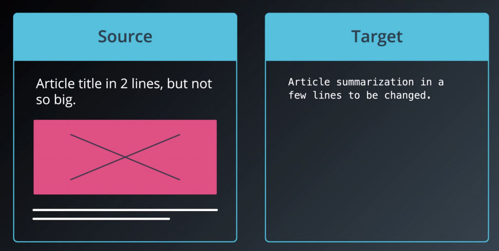
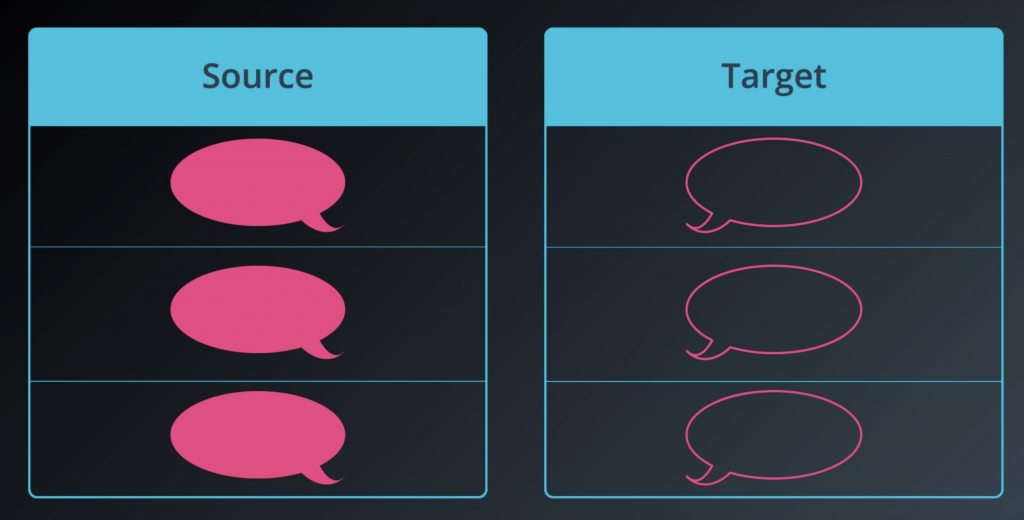
The term sequence-to-sequence RNN is a little bit abstract and doesn’t relay how many amazing things we can do with this type of model. So let’s think of it like this. We have a model that can learn to generate any sequence of vectors. And these can be letters. They can be words or images or anything, really. If you can represent it as a vector, it can be used in a sequence-to-sequence model. So this model can learn to generate any sequence of vectors after we feed. Say you train it on a dataset where the source is an English phrase and the target is a French phrase. And you have a lot of these examples. If you do that and you train it successfully, then your model is now in English-to-French translator.

Train it on a dataset of news articles and their summaries and you have a summarization bot.

Train it on a dataset of questions and their answers and you have a question-answering model.

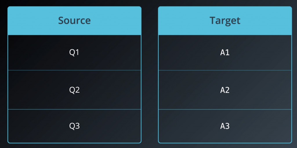
Train it on a lot of dialogue data and you have a chatbot.

Let’s look more closely at how sequence to sequence models work. We got two recurrent nets

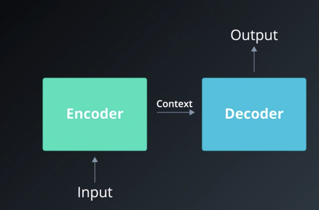
The one on the left is called the encoder. It reads the input sequence, then hands over what it has understood to the RNN and on the right, which we call the decoder. And the decoder generates the output sequence.

The context is the last hidden state of encoder. No matter how short or long
the inputs and outputs are, the context remains the same size

Now if we go a level deeper, we begin to see that since the encoder and decoder are both RNNs, they have loops, naturally, and that’s what allows them to process these sequences of inputs and outputs.

Say our model want to ask it, “How are you,” question mark.

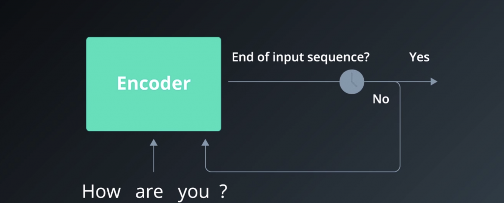
So first, we have to tokenize that input, and break it down into four tokens. And since it has four elements, it will take the RNN
four timesteps to read in this entire sequence. Each time, it would read an input, and then do a transformation on its hidden state, then send that hidden state out to the next time step.

One useful way to represent the flow of data through an RNN is by “unrolling” the RNN.

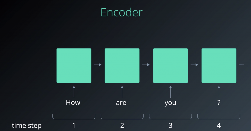
So, what’s a hidden state, you may ask?. In the simplest scenario, you can think of it as a number of hidden units inside the cell. The bigger the hidden states, and the bigger the size, the more capacity of the model

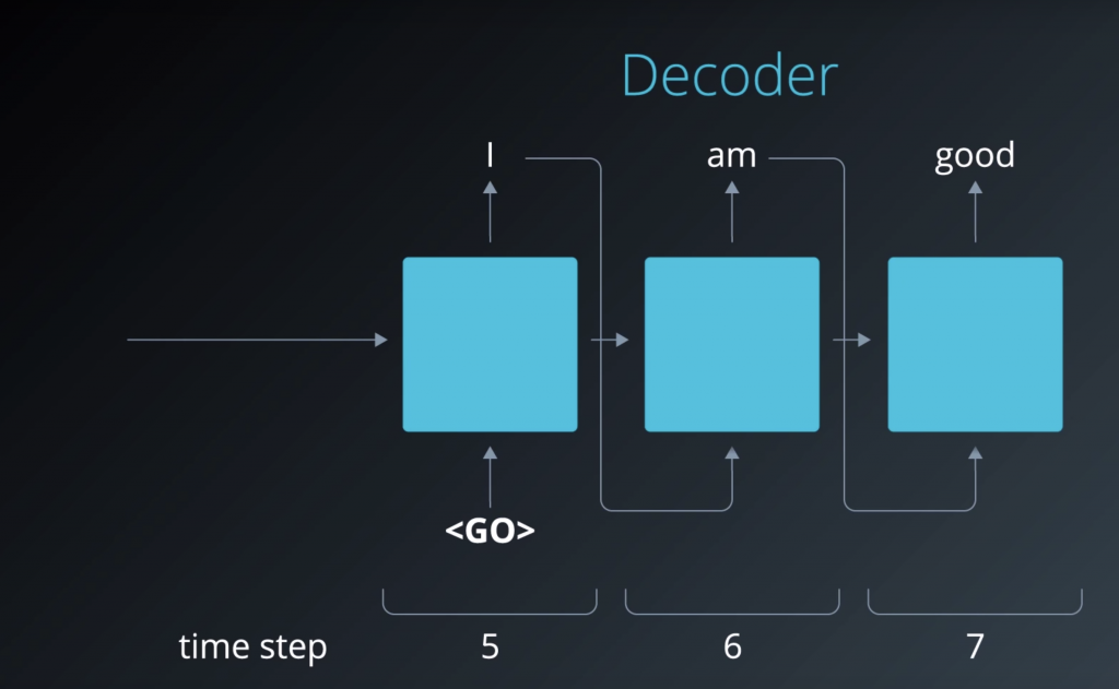
A similar process happens on the decoder side, as well. So we begin by feeding it this
data generated by the encoder. And it generates the output elements by elements. If we unroll the decoder, just like we did earlier with the encoder, so we can see that we are actually feeding it back every element that it outputs.

Encoding — Attention Overview

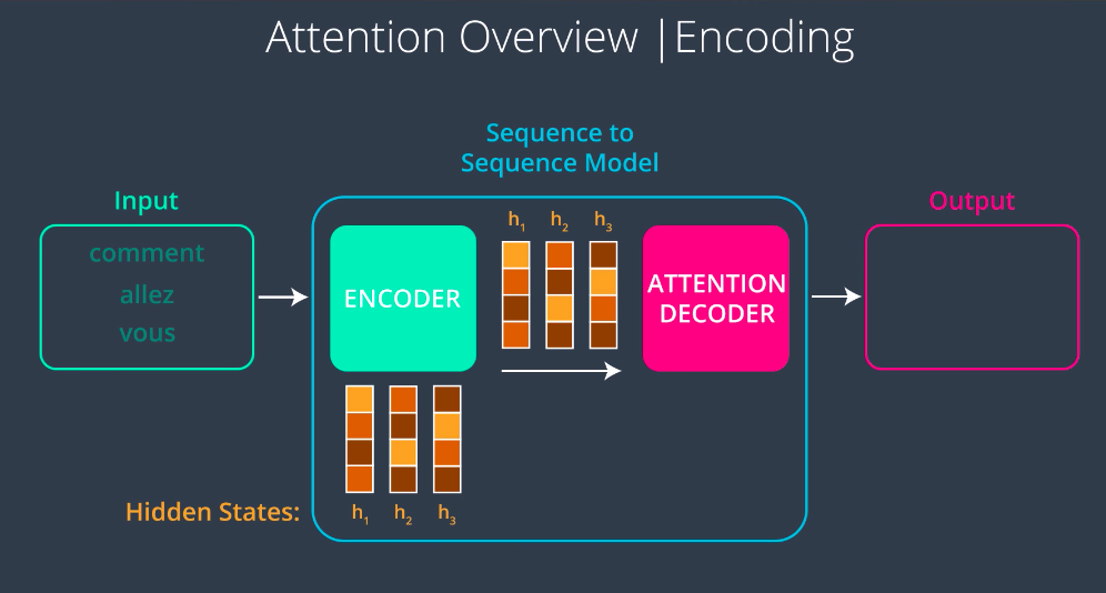
A Sequence to Sequence Model with attention works in the following way. First, the encoder processes the input sequence just like the model without attention one word at a time, producing a hidden state and using that hidden state and the next step. Next, the model passes a context vector to the decoder but unlike the context vector in the model without attention, this one is not just the final hidden state it’s all of the hidden states. This gives us the benefit of having the flexibility in the context size.

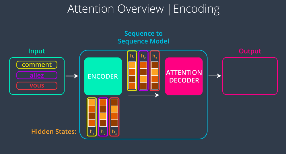
The first hidden state was outputted after processing the first word, so it captures the essence of the first word the most. So when we focus on this vector, we will be focusing on that word the most, the same with the second hidden state with the second word etc …

Decoding — Attention Overview

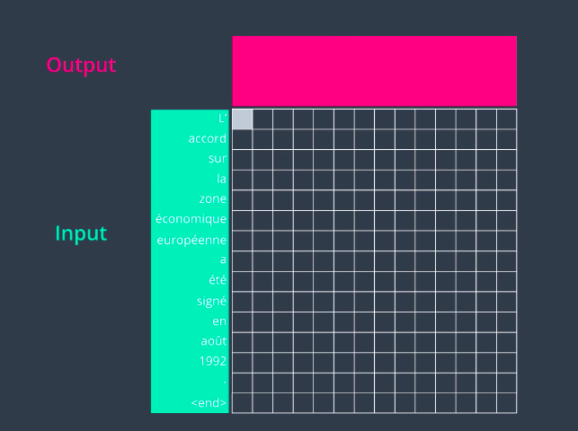
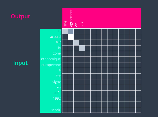
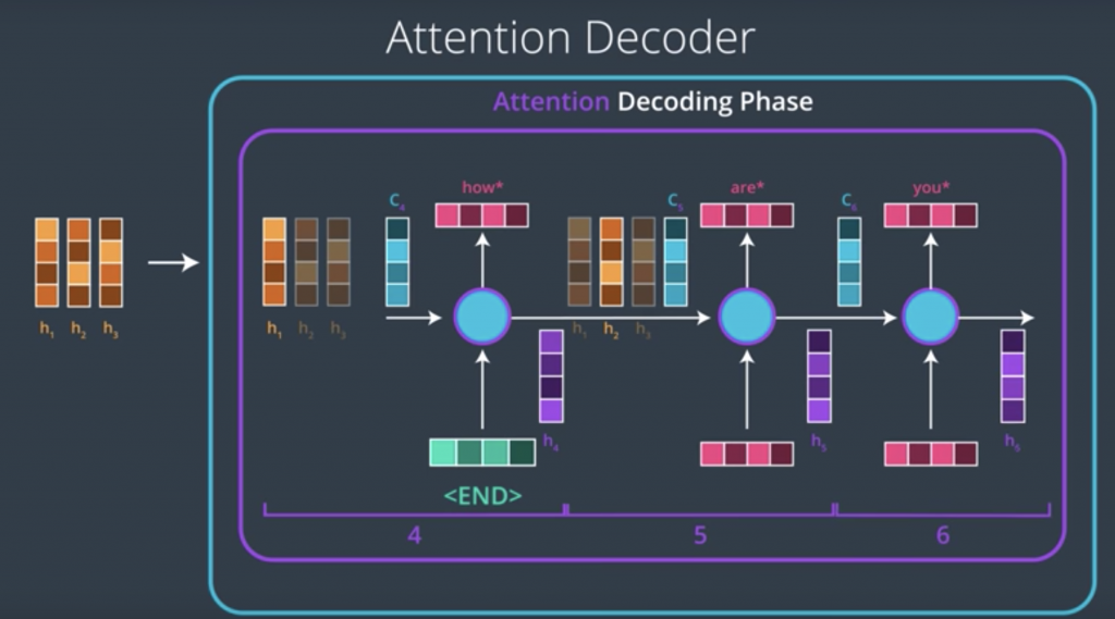
Now, let’s look at the attention decoder and how it works at a very high level. At every time step, an attention decoder pays attention to the appropriate part of the input sequence using the context factor. How does the attention decoder know which of the parts of the input sequence to focus on at each step? That process is learned during the training phase, and it’s not just stupidly going sequentially from the first and the second to the third. It can learn some sophisticated behavior. Let’s look at this example of translating a French sentence to an English one. So let’s say we have this input sentence in French. Let’s say we pass this to our encoder and now we’re ready to look at each step in the decoding phase. In the first step, the attention decoder would pay attention to the first part of the sentence. This is a trained model So the more light the square is is the more attention that he gave to that word in particular. So it pays attention to the first word and it outputs a first English word.

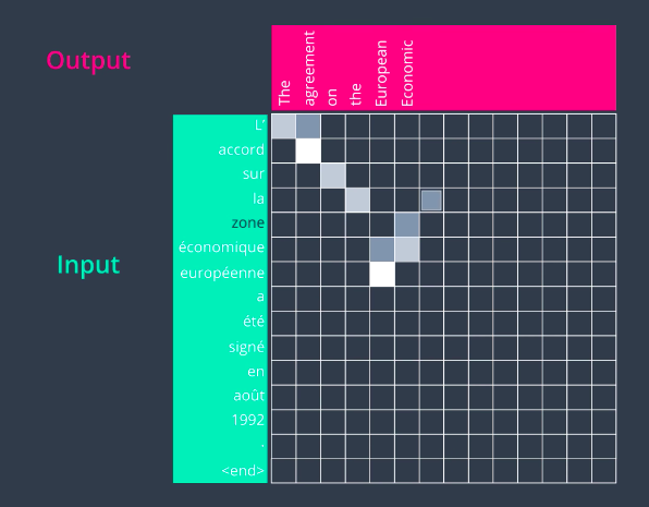
In the second step, it pays attention to the second word in the input sequence and translates that word as well. It goes on sequentially for about four steps and it produces reasonable English translation so far.

Then something different happens here in the fifth step. So, when we’re generating the fifth word of the output, the attention actually jumped two words to translate European. So, we have zone, economique, europeenne, so on the English side it’s not going to be in the same order. So, europeenne is translated as European and then in the next step it focuses on the word before that, economique, economic, and it focuses on zone and it outputs area. This is a case where the order of these words in the French language does not follow how it would be ordered in the English language and the model was able to learn that just from a training data set.

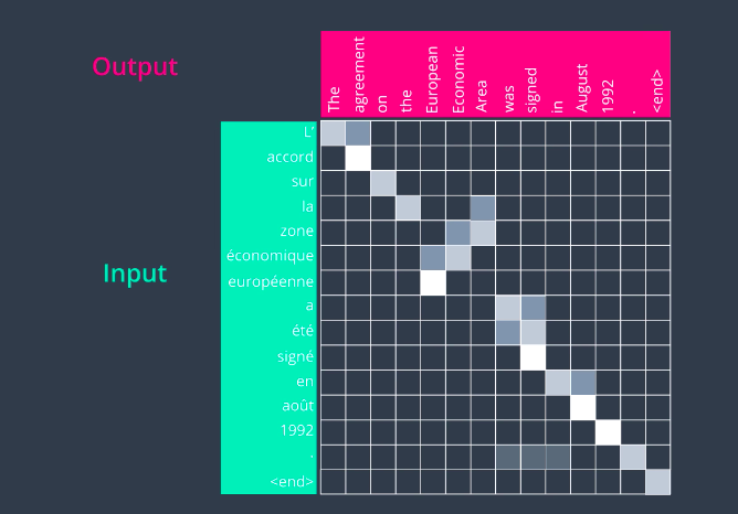
The rest of the sentence goes on pretty much sequentially.

Attention Encoder

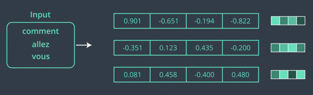
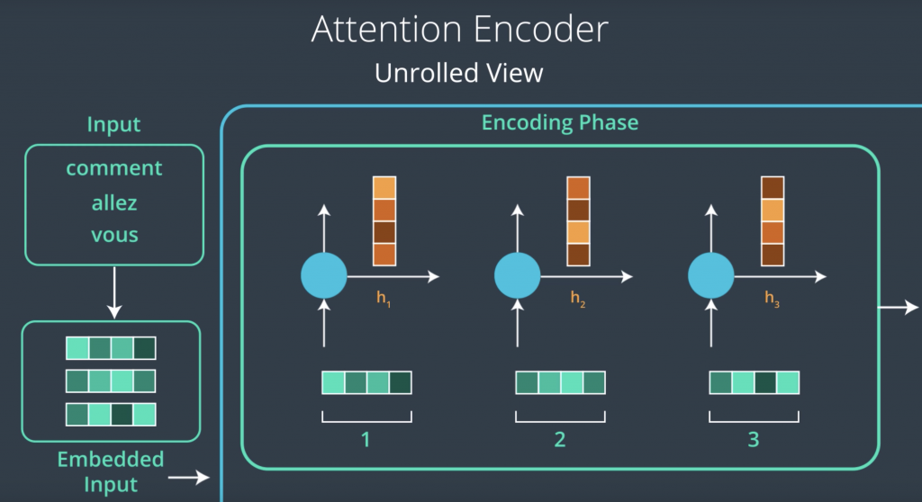
Now that we’ve taken a high level look at how attention works in a sequence to sequence model, let’s look into it in more detail. We’ll use machine translation as the example as that’s the application the main papers on attention tackled. But whatever we do here, translates into other applications as well. It’s important to note that there is a small variety of attention algorithms. We’ll be looking at a simple one here. Let’s start from the Encoder. In this example, the Encoder is a recurrent neural network. When creating an RNN, we have to declare the number of hidden units in the RNN cell. This applies whether we have a vanilla RNN or an LSTM or GRU cell. Before we start feeding our input sequence words to the Encoder, they have to pass through an embedding process which translates each word into a vector. Here we can see the vector representing each of these words. Now, this is a toy embedding of size four just for the purpose of easier visualization. In real-world applications, a size like 200 or 300 is more appropriate.

Now that we have our words and their embeddings, we’re ready to feed that into our Encoder. Feeding the first word into the first time step of the RNN produces the first hidden state. This is what’s called an unrolled view of the RNN, where we can see the RNN at each time step. We’ll hold onto this state and the RNN would continue to process the next time step. So, it would take the second word and pass it to the RNN at the second time step, and then it would do that with the third word as well. Now that we have processed the entire input sequence, we’re ready to pass the hidden states to the attention decoder.

Attention Decoder

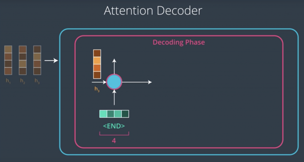
Let’s now look at things on the decoder side. In models without attention, we’d only feed the last context vector to the decoder RNN, in addition to the embedding of the end token, and it will begin to generate an element of the output sequence at each time-step. The case is different in an attention decoder, however. An attention decoder has the ability to look at the inputted words, and the decoders own hidden state,

and then it would do the following. It would use a scoring function to score each hidden state in the context matrix. After scoring each context vector would end up with a certain score and if we feed these scores into a softmax function, we end up with scores that are all positive, that are all between zero and one, and that all sum up to one. These values are how much each vector will be expressed in the attention vector that the decoder will look at before producing an output.

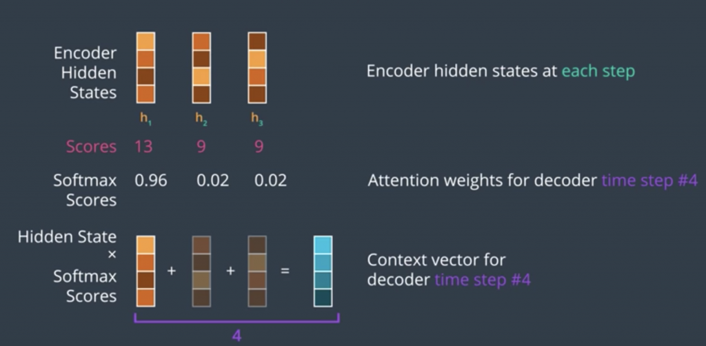
Simply multiplying each vector by its softmax score and then, summing up these vectors produces an attention contexts vector, this is a basic weighted sum operation. The context vector is an important milestone in this process, The decoder has now looked at the input word and at the attention context vector, which focused its attention on the appropriate place in the input sequence.

Bahdanau and Luong Attention

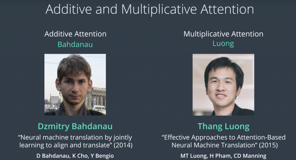
Before delving into the details of scoring functions, we need to make a distinction of the two major types of attention. These are often referred to as “Additive Attention and Multiplicative Attention.” Sometimes they’re also called “Bahdanau Attention” and “Luong Attention,” referring to the first authors of the papers, which described them.

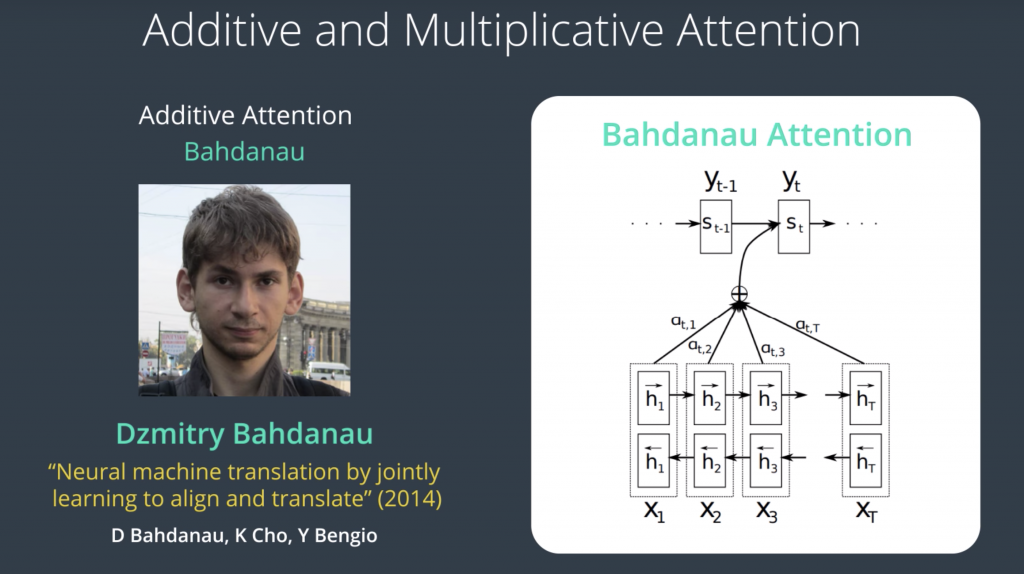
The scoring function in Bahdanau attention looks like this

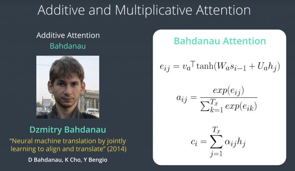
where h of j is the hidden state from the encoder, s of i minus one is the hidden state of the decoder in the previous time step. u of a, W of a, and v of a, are all weight matrices that are learned during the training process. Basically, this is a scoring function, which takes the hidden state of the encoder, hidden state of the decoder and produces a single number for each decoder time step. The scores are then passed into softmax, and then this is our weighted sum operation, where we multiply each encoder hidden state, by its score, and then we sum them all up, producing our attention context vector.

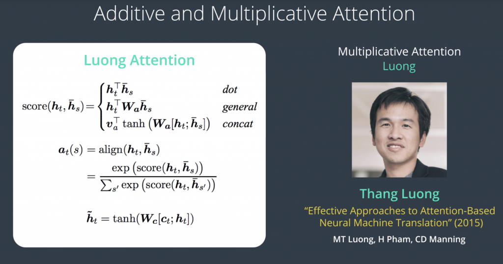
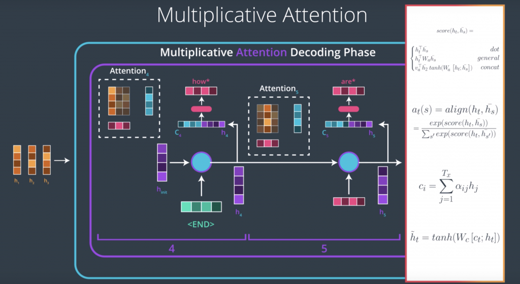
Multiplicative attention or Luong attention referring to Thang Luong, the first author of the paper, Luong attention built on top of the Bahdanau attention by adding a couple more scoring function. Their architecture is also different and that they used only the hidden states from the top RNN layer in the encoder. This allows the encoder and the decoder to both be stacks of RNNs, which led to some of the premier models that are in production right now.

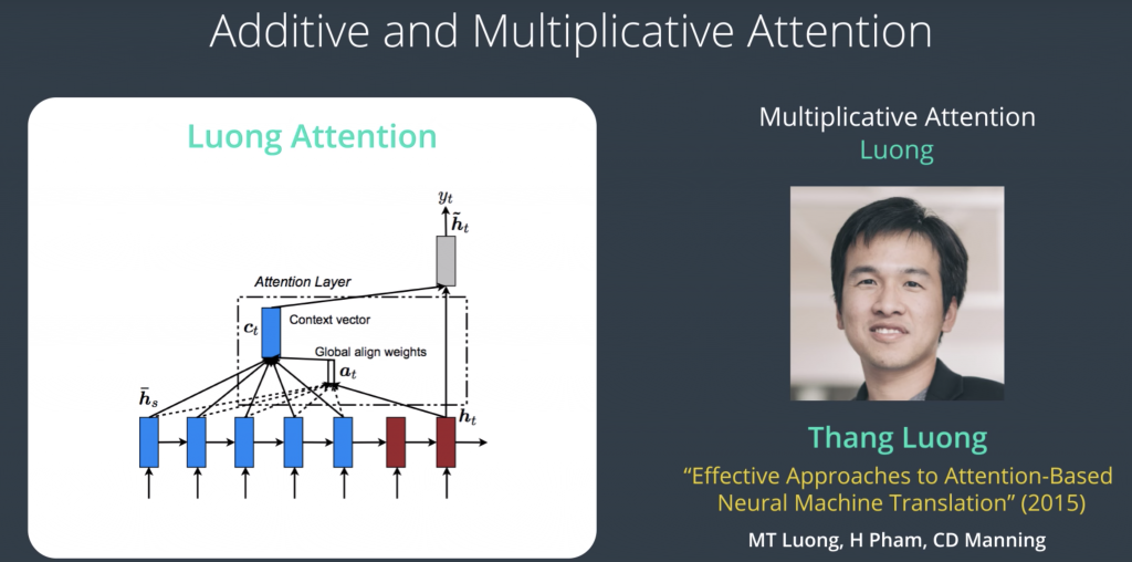
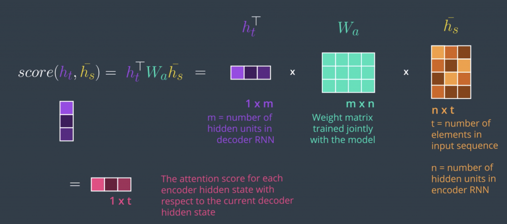
The scoring functions in multiplicative attention are three that we can choose from The simplest one is the dot scoring function, which is multiplying the hidden states of the encoder by the hidden state of the decoder. The second scoring function is called general, it builds on top of it and just adds a weight matrix between them, and this multiplication in the dot product is where multiplicative attention gets its name. The third is very similar to Bahdanau attention, in that it adds up the hidden state of the encoder with the hidden state of the decoder, and so this addition is where additive attention gets its name, then multiplies it by a weight matrix, applies a tanh activation and then multiplies it by another weight matrix. So, this is a function that we give the hidden state of the decoder at this time step and the hidden states of the encoder at all the time steps, and it will produce a score for each one of them. We then do softmax just as we did before, and then that would produce c of t here, they are called the attention context vector

Multiplicative Attention

An attention scoring function tends to be a function that takes in the hidden state of the decoder and the set of hidden states of the encoder. Since this is something we’ll do at each timestep on the decoder side, we only use the hidden state of the decoder at that timestep or the previous timestep in some scoring methods.

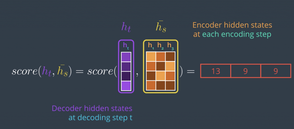
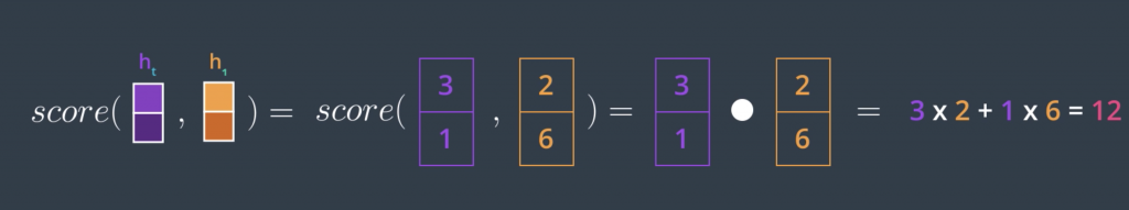
Given these two inputs, this vector and this matrix, it produces a vector that scores each of these columns. Before looking at the matrix version, which calculates the scores for all the encoder hidden states in one step, let’s simplify it by looking at how to score a single encoder hidden state. The first scoring method and the simplest is to just calculate the dot product of the two input vectors. The dot product of two vectors produces a single number, so that’s good.

But the important thing is the significance of this number. Geometrically, the dot product of two vectors is equal to multiplying the lengths of the two vectors by the cosine of the angle between them, and we know that cosine has his convenient property that it equals one if the angle is zero and it decreases,

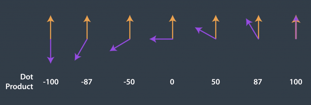
This dot product is a similarity measure between vectors. The dot product produces a larger number, the smaller the angle between the vectors are.

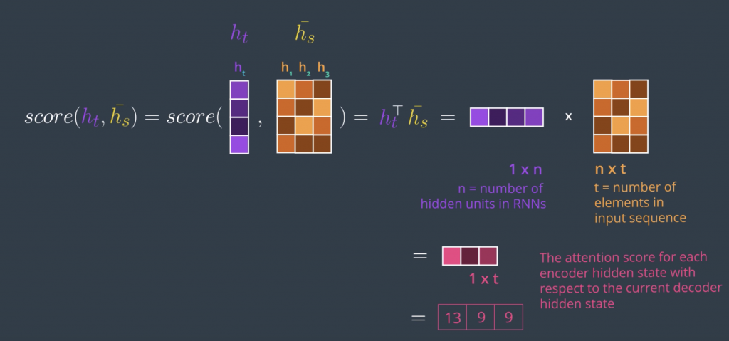
In practice, however, we want to speed up the calculation by scoring all the encoder hidden states at once, which leads us to the formal mathematical definition of dot product attention which leads us to the formal mathematical definition of dot product attention.

With the simplicity of this method comes the drawback of assuming the encoder and decoder have the same embedding space. So, while this might work for text summarization, for example, where the encoder and decoder use the same language and the same embedding space. For machine translation, however, you might find that each language tends to have its own embedding space. This is a case where we might want to use the second scoring method,

Let us now look back at this process and incorporate everything that we know about attention.

Additive Attention

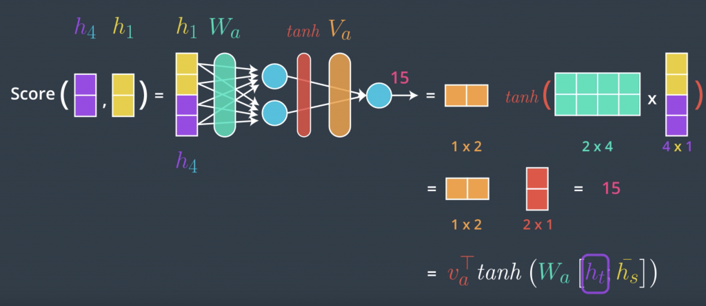
we’ll look at the third commonly used scoring method It’s called concat, and the way to do it is to use a feedforward neural network. To take a simple example, let’s say we’re scoring this encoder hidden state at the fourth time step at the decoder. Again this is an oversimplified example scoring only one, while in practice we’ll actually do a matrix and do it all discord in one step. The concat scoring method, is commonly done by concatenating the two vectors, and making that the input to a feed forward neural network. Let’s see how that works. So, we merge them, we concat them into one vector, and then we pass them through a neural network. This network has a single hidden layer, and outputs this score. The parameters of this network are learned during the training process.

An sample notebook for machine translation with attention in pytorch can be found at
http://14.232.166.121:8880/lab/workspaces/andy > attention > attention.ipynb