RNN

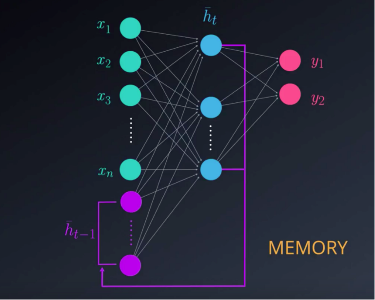
if you look up the definition of the word Recurrent, you will find that it simply means occurring often or repeatedly. So why are these networks called Recurrent Neural Networks? It’s simply because with RNN’s, we perform the same task for each element in the input sequence. RNN’s also attempt to address the need for capturing information and previous inputs by maintaining internal memory elements, also known as States.

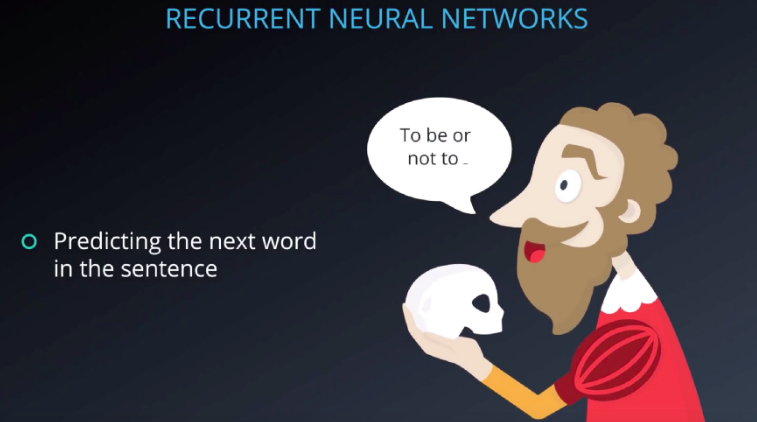
Many applications have temporal dependencies. Meaning, that the current output depends not only on the current input, but also on a memory element which takes into account past inputs. For cases like these, we need to use RNN’s. A good example for the use of RNN is predicting the next word in a sentence, which typically requires looking at the last few words rather than only the current one.

so how should we think about this new neural network?, How are the training, and evaluation phases changed? RNN’s are based on the same principles behind feedforward neural networks. In the RNN network, the inputs and outputs can also be many-to-many, many-to-one, and one-to-many. There are however, two fundamental differences between RNN’s, and feedforward neural networks. The first, is the manner by which we define our inputs and outputs. Instead of training the network using a single-input, single-output at each time step, we train with sequences since previous inputs matter. The second difference, stems from the memory elements that RNN’s host. Current inputs, as well as activations of neurons serve as inputs to the next time step.

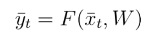
As we’ve see, in FFNN the output at any time t, is a function of the current input and the weights. This can be easily expressed using the following equation:

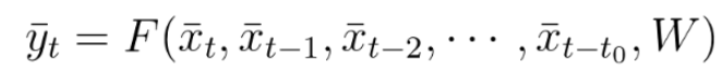
In RNNs, our output at time t, depends not only on the current input and the weight, but also on previous inputs. In this case the output at time t will be defined as:

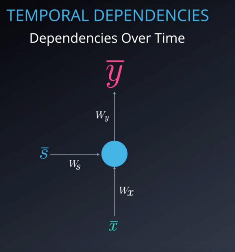
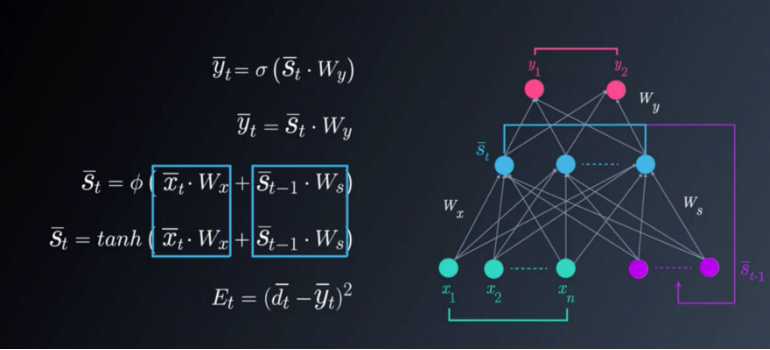
This is the RNN folded model:

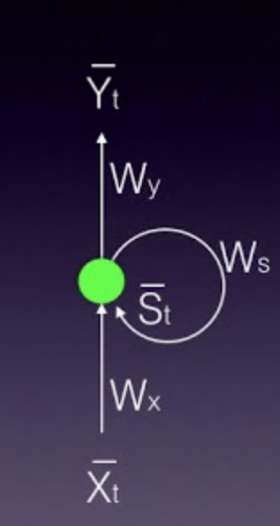
In this picture, “x bar “represents the input vector, “y bar”​ represents the output vector and “s bar” denotes the state vector.

Wx​ is the weight matrix connecting the inputs to the state layer.

Wy​ is the weight matrix connecting the state layer to the output layer.

Ws​ represents the weight matrix connecting the state from the previous timestep to the state in the current timestep.

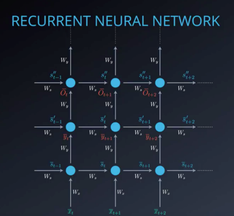
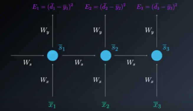
The model can also be “unfolded in time”. The unfolded model is usually what we use when working with RNNs.

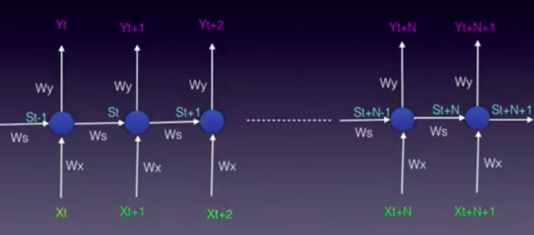
In both the folded and unfolded models shown above the following notation is used:

“x bar” represents the input vector, “y bar” represents the output vector and “s bar”represents the state vector.

Wx​ is the weight matrix connecting the inputs to the state layer.

Wy​ is the weight matrix connecting the state layer to the output layer.

Ws​ represents the weight matrix connecting the state from the previous time-step to the state in the current time-step.

In FFNNs the hidden layer depended only on the current inputs and weights, as well as on an activation function Φ in the following way:

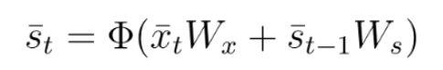
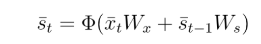
In RNNs the state layer depended on the current inputs, their corresponding weights, the activation function and also on the previous state:

The output vector is calculated exactly the same as in FFNNs. It can be a linear combination of the inputs to each output node with the corresponding weight matrix Wy​, or a softmax function of the same linear combination.

Backpropagation Through Time (BPTT)

Before diving into Backpropagation Through Time we need a few reminders.

The state vector “s t bar”​ is calculated the following way:

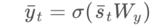
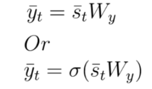
The output vector “y t bar”​ can be product of the state vector “st bar”​ and the corresponding weight elements of matrix Wy​. As mentioned before, if the desired outputs are between 0 and 1, we can also use a softmax function. The following set of equations depicts these calculations:

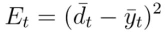
As mentioned before, for the error calculations we will use the Loss Function, where

Et​ represents the output error at time t

dt​ represents the desired output at time t

yt​ represents the calculated output at time t

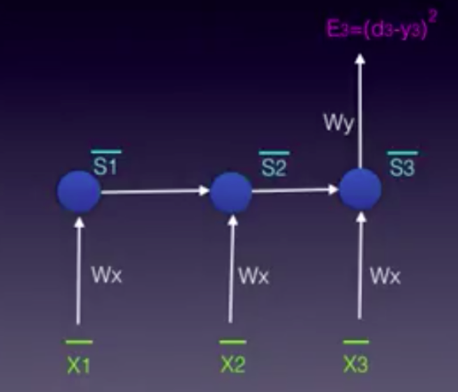
In BPTT we train the network at timestep t as well as take into account all of the previous timesteps. The easiest way to explain the idea is to simply jump into an example. In this example we will focus on the BPTT process for time step t=3. You will see that in order to adjust all three weight matrices,Wx​,Ws​ and Wy​, we need to consider timestep 3 as well as timestep 2 and timestep 1.

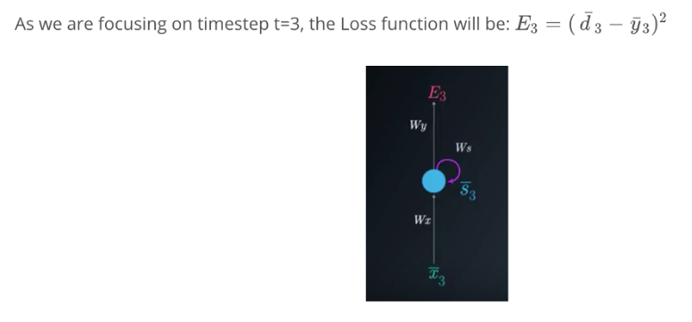
To update each weight matrix, we need to find the partial derivatives of the Loss Function at time 3, as a function of all of the weight matrices. We will modify each matrix using gradient descent while considering the previous timesteps.

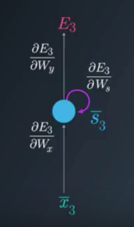
The unfolded model can be very helpful in visualizing the BPTT process.

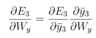
The partial derivative of the Loss Function with respect to Wy​ is found by a simple one step chain rule: (Note that in this case we do not need to use BPTT)

Gradient calculations needed to adjust Wy​

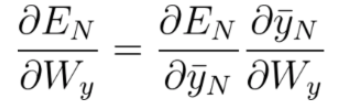
Generally speaking, we can consider multiple timesteps back, and not only 3 as in this example. For an arbitrary timestep N, the gradient calculation needed for adjusting Wy​, is:

Gradient calculations needed to adjust Ws

We still need to adjust Ws​ the weight matrix connecting one state to the next and Wx​ the weight matrix connecting the input to the state. We will arbitrarily start with Ws​.

To understand the BPTT process, we can simplify the unfolded model. We will focus on the contributions of Ws​ to the output, the following way:

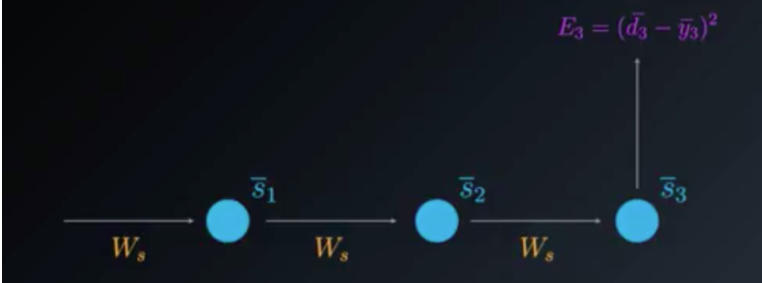
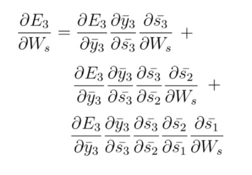
​n BPTT we will take into account every gradient stemming from each state, accumulating all of these contributions.

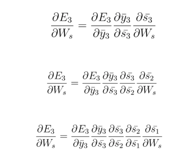
The following equation is the gradient contributing to the adjustment of Ws​ using Backpropagation Through Time:

Gradient calculations needed to adjust Wx​

To further understand the BPTT process, we will simplify the unfolded model again. This time the focus will be on the contributions of W_xWx​ to the output, the following way:

As we mentioned previously, in BPTT we will take into account each gradient stemming from each state, accumulating all of the contributions.

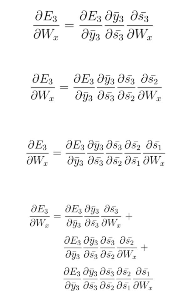
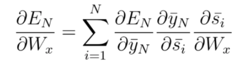
in this example we had 3 time steps to consider, therefore we accumulated three partial derivative calculations. Generally speaking, we can consider multiple timesteps back. If you look closely at equations 1, 2 and 3, you will notice a pattern again. You will find that as we propagate a step back, we have an additional partial derivatives to consider in the chain rule. Mathematically this can be easily written in the following general equation for adjusting Wx​ using BPTT:

the sample for RNN can be found at http://14.232.166.121:8880/lab?

andy > rnn >Simple_RNN.ipynb

you should shut down the kernel after running experiment 😀