Training Optimization

So by now we’ve learned how to build a deep neural network and how to train it to fit our data. Sometimes however, we go out there and train on ourselves and find out that nothing works as planned. Why? Because there are many things that can fail. Our architecture can be poorly chosen, our data can be noisy, our model could maybe be taking years to run and we need it to run faster. We need to learn ways to optimize the training of our models and this is what we’ll do next.

Testing

So let’s look at the following data form by blue and red points, and the following two classification models which separates the blue points from the red points. The question is which of these two models is better?

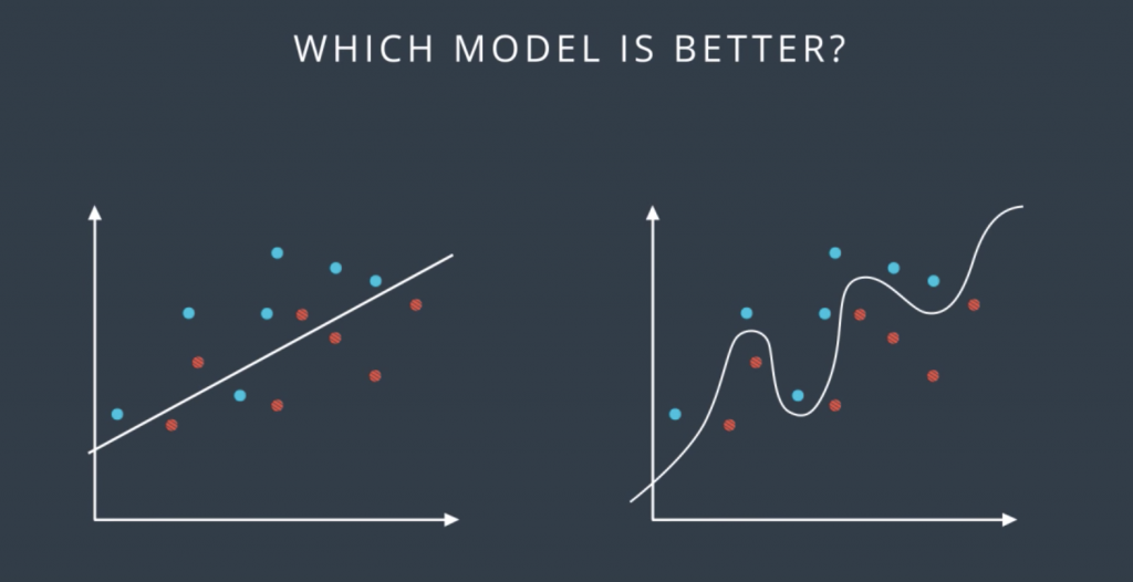
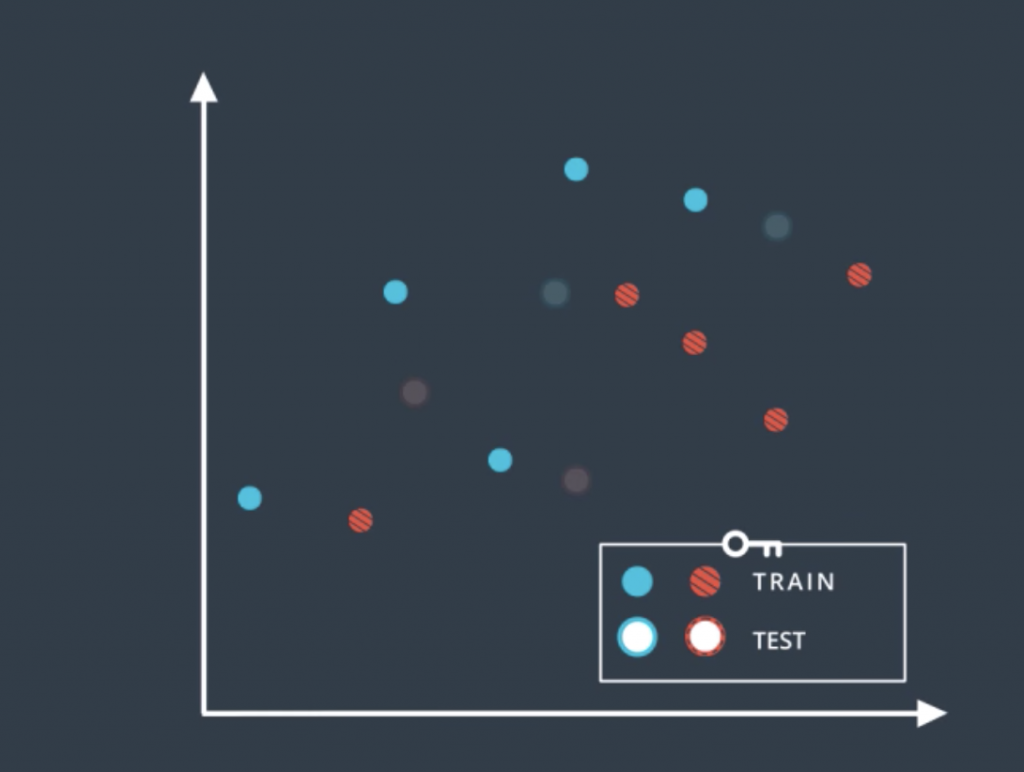
Well, it seems like the one on the left is simpler since it’s a line and the one on the right is more complicated since it’s a complex curve. Now the one in the right makes no mistakes. It correctly separates all the points, on the other hand, the one in the left does make some mistakes. So we’re inclined to think that the one in the right is better. In order to really find out which one is better, we introduce the concept of training and testing sets. We’ll denote them as follows: the solid color points are the training set, and the points with the white inside are the testing set. And what we’ll do is we’ll train our models in the training set without looking at the testing set, and then we’ll evaluate the results on that testing to see how we did.

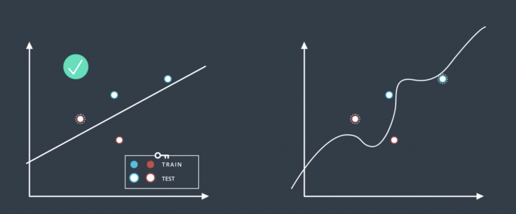
So according to this, we trained the linear model and the complex model on the training set to obtain these two boundaries. Now we reintroduce the testing set and we can see that the model in the left made one mistake while the model in the right made two mistakes. So in the end, the simple model was better. Does that match our intuition?. Well, it does, because in machine learning that’s what we’re going to do. Whenever we can choose between a simple model that does the job and a complicated model that may do the job a little bit better, we always try to go for the simpler model.

Overfitting and Underfitting

So, let’s talk about life. In life, there are two mistakes one can make. One is to try to kill Godzilla using a flyswatter. The other one is to try to kill a fly using a bazooka.

What’s the problem with trying to kill Godzilla with a flyswatter? That we’re oversimplifying the problem. We’re trying a solution that is too simple and won’t do the job. In machine learning, this is called underfitting. And what’s the problem with trying to kill a fly with a bazooka? It’s overly complicated and it will lead to bad solutions and extra complexity when we can use a much simpler solution instead. In machine learning, this is called overfitting Let’s look at how overfitting and underfitting can occur in a classification problem. Let’s say we have the following data, and we need to classify it.

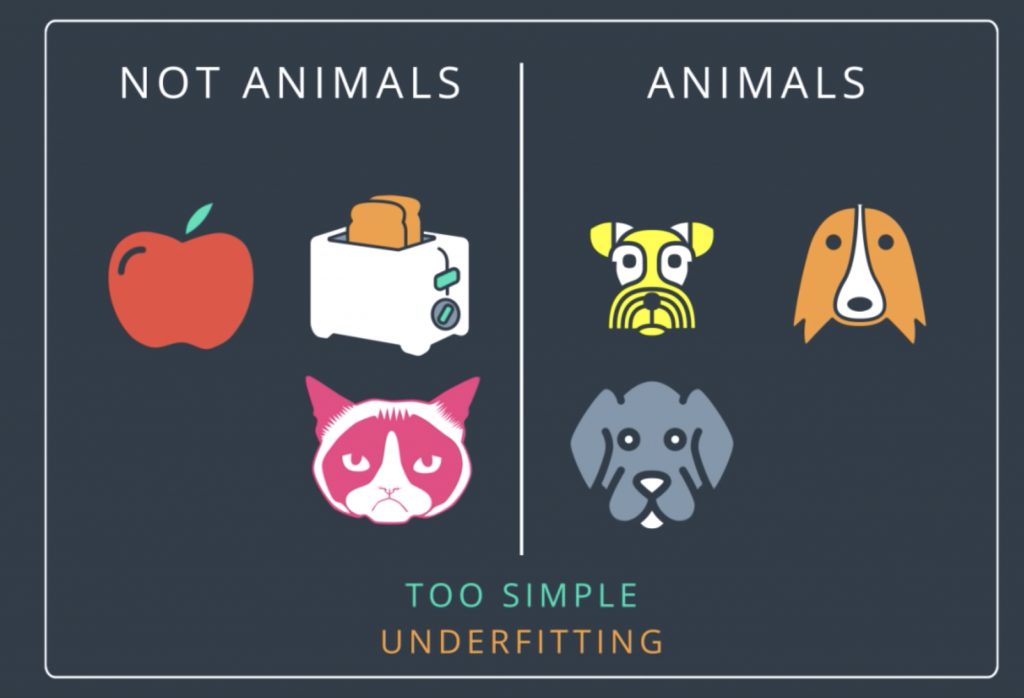
So what is the rule that will do the job here? Seems like an easy problem, right? The ones in the right are dogs while the ones in the left are anything but dogs. Now what if we use the following rule? We say that the ones in the right are animals and the ones in the left are anything but animals. Well, that solution is not too good, right? What is the problem? It’s too simple. It doesn’t even get the whole data set right. See? It misclassified this cat over here since the cat is an animal. This is underfitting.

Now, what about the following rule? We’ll say that the ones in the right are dogs that are yellow, orange, or grey, and the ones in the left are anything but dogs that are yellow, orange, or grey. Well, technically, this is correct as it classifies the data correctly. There is a feeling that we went too specific since just saying dogs and not dogs would have done the job. But this problem is more conceptual, right? How can we see the problem here? Well, one way to see this is by introducing a testing set. If our testing set is this dog over here, then we’d imagine that a good classifier would put it on the right with the other dogs. But this classifier will put it on the left since the dog is not yellow, orange, or grey. So, the problem here, as we said, is that the classifier is too specific. It will fit the data well but it will fail to generalize. This is overfitting.

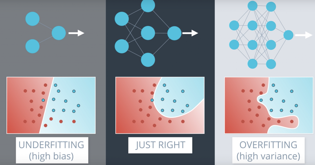
But now, let’s see how this would look like in neural networks. So let’s say this data where, again, the blue points are labeled positive and the red points are labeled negative. And here, we have the three little bears. In the middle, we have a good model which fits the data well. On the left, we have a model that underfits since it’s too simple. It tries to fit the data with the line but the data is more complicated than that. And on the right, we have a model that overfits since it tries to fit the data with an overly complicated curve. Notice that the model in the right fits the data really well since it makes no mistakes, whereas the one in the middle makes this mistake over here. But we can see that the model in the middle will probably generalize better. The model in the middle looks at this point as noise. while the one in the right gets confused by it and tries to feed it too well. Now the model in the middle will probably be a neural network with a slightly complex architecture like this one.

Early Stopping

So, let’s start from where we left off, which is, we have a complicated network architecture which would be more complicated than we need but we need to live with it. So, let’s look at the process of training. We start with random weights in her first epoch and we get a model like this one, which makes lots of mistakes. Now as we train, let’s say for 20 epochs we get a pretty good model. But then, let’s say we keep going for a 100 epochs, we’ll get something that fits the data much better, but we can see that this is starting to over-fit. If we go for even more, say 600 epochs, then the model heavily over-fits. We can see that the blue region is pretty much a bunch of circles around the blue points. This fits the training data really well, but it will generalize horribly. Imagine a new blue point in the blue area. This point will most likely be classified as red unless it’s super close to a blue point.

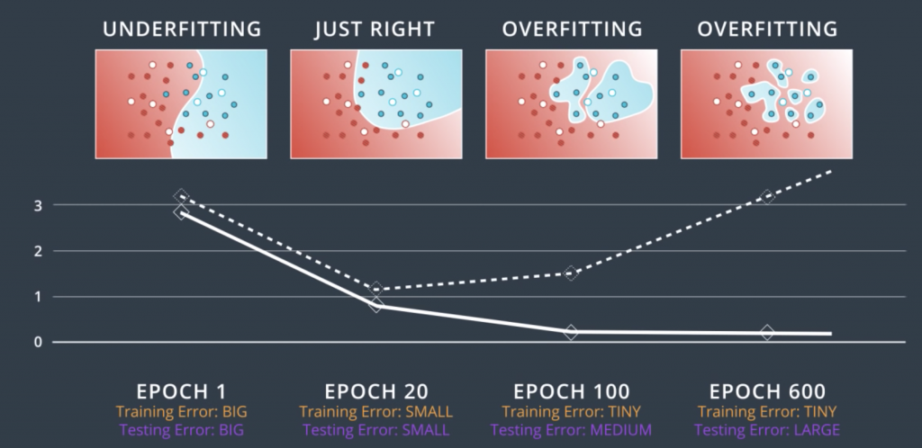
So, let’s try to evaluate these models by adding a testing set such as these points. Let’s make a plot of the error in the training set and the testing set with respect to each epoch. For the first epoch, since the model is completely random, then it badly misclassifies both the training and the testing sets. So, both the training error and the testing error are large. We can plot them over here. For the 20 epoch, we have a much better model which fit the training data pretty well, and it also does well in the testing set. So, both errors are relatively small and we’ll plot them over here. For the 100 epoch, we see that we’re starting to over-fit. The model fits the data very well but it starts making mistakes in the testing data. We realize that the training error keeps decreasing, but the testing error starts increasing, so, we plot them over here. Now, for the 600 epoch, we’re badly over-fitting.

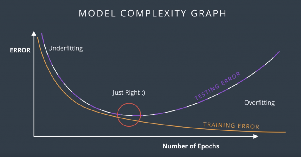
Now, we draw the curves that connect the training and testing errors. So, in this plot, it is quite clear when we stop under-fitting and start over-fitting, the training curve is always decreasing since as we train the model, we keep fitting the training data better and better. The testing error is large when we’re under-fitting because the model is not exact. Then it decreases as the model generalizes well until it gets to a minimum point – the Goldilocks spot. And finally, once we pass that spot, the model starts over-fitting again since it stops generalizing and just starts memorizing the training data. This plot is called the model complexity graph.

Regularization

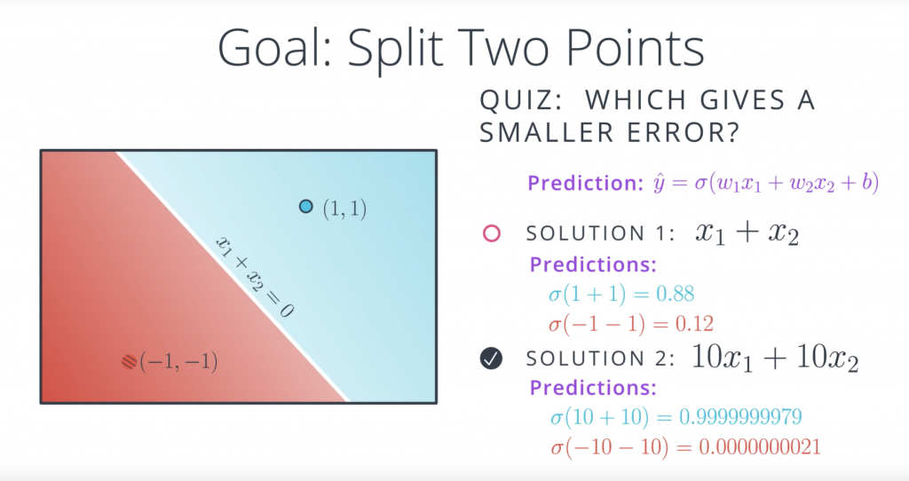
Well the first observation is that both equations give us the same line, the line with equation X1+X2=0. And the reason for this is that solution two is really just a scalar multiple of solution one. So let’s see. Recall that the prediction is a sigmoid of the linear function. So in the first case, for the 0.11, it would be sigmoid of 1+1, which is sigmoid of 2, which is 0.88. This is not bad since the point is blue, so it has a label of one. For the point (-1, -1), the prediction is sigmoid of -1+-1, which is sigmoid of -2, which is 0.12. It’s also not best since a point label has a label of zero since it’s red. Now let’s see what happens with the second model. The point (1, 1) has a prediction sigmoid of 10 times 1 plus 10 times 1 which is sigmoid of 20. This is a 0.9999999979, which is really close to 1, so it’s a great prediction. And the point (-1, -1) has prediction sigmoid of 10 times negative one plus 10 times negative one, which is sigmoid of minus 20, and that is 0.0000000021. That’s a really, really close to zero so it’s a great prediction. So the answer to the quiz is the second model,

the second model is super accurate. This means it’s better, right? Well after the last section you may be a bit reluctant since this hint’s a bit towards overfitting. And your hunch is correct. The problem is overfitting but in a subtle way. Here’s what’s happening and here’s why the first model is better even if it gives a larger error.

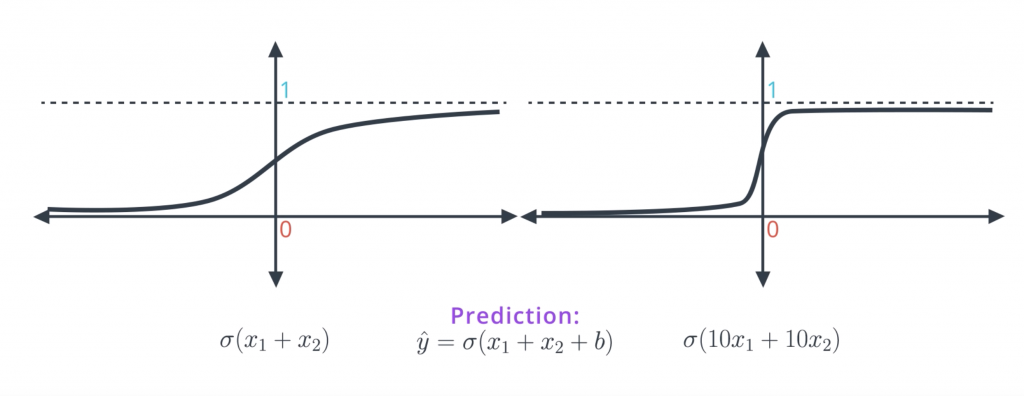
When we apply sigmoid to small values such as X1+X2, we get the function on the left which has a nice slope to the gradient descent. When we multiply the linear function by 10 and take sigmoid of 10X1+10X2, our predictions are much better since they’re closer to zero and one. But the function becomes much steeper and it’s much harder to do great descent here. Since the derivatives are mostly close to zero and then very large when we get to the middle of the curve. Therefore, in order to do gradient descent properly, we want a model like the one in the left more than a model like the one in the right. In a conceptual way the model in the right is too certain and it gives little room for applying gradient descent. Also as we can imagine, the points that are classified incorrectly in the model in the right, will generate large errors and it will be hard to tune the model to correct them.

Now the question is, how do we prevent this type of overfitting from happening? This seems to not be easy since the bad model gives smaller errors. Well, all we have to do is we have to tweak the error function a bit. Basically we want to punish high coefficients. So what we do is we take the old error function and add a term which is big when the weights are big. There are two ways to do this. One way is to add the sums of absolute values of the weights times a constant lambda. The other one is to add the sum of the squares of the weights times that same constant. As you can see, these two are large if the weights are large. The lambda parameter will tell us how much we want to penalize the coefficients. If lambda is large, we penalized them a lot. And if lambda is small then we don’t penalize them much. And finally, if we decide to go for the absolute values, we’re doing L1 regularization and if we decide to go for the squares, then we’re doing L2 regularization.

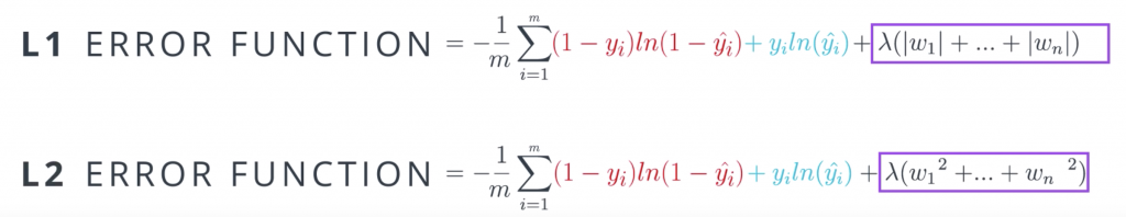
Here are some general guidelines for deciding between L1 and L2 regularization. When we apply L1, we tend to end up with sparse vectors. That means, small weights will tend to go to zero. So if we want to reduce the number of weights and end up with a small set, we can use L1. This is also good for feature selections and sometimes we have a problem with hundreds of features, and L1 regularization will help us select which ones are important, and it will turn the rest into zeroes. L2 on the other hand, tends not to favor sparse vectors since it tries to maintain all the weights homogeneously small

Dropout

This is something that happens a lot when we train neural networks. Sometimes one part of the network has very large weights and it ends up dominating all the training, while another part of the network doesn’t really play much of a role so it doesn’t get trained. So, what we’ll do to solve this is sometimes during training, we’ll turn this part off and let the rest of the network train.

More thoroughly, what we do is as we go through the epochs, we randomly turn off some of the nodes and say, you shall not pass through here. In that case, the other nodes have to pick up the slack and take more part in the training.

Vanishing Gradient

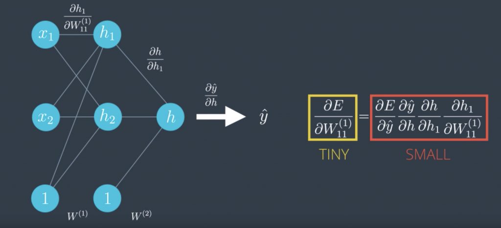
Here’s another problem that can occur. Let’s take a look at the sigmoid function. The curve gets pretty flat on the sides. So, if we calculate the derivative at a point way at the right or way at the left, this derivative is almost zero.This is not good cause a derivative is what tells us in what direction to move. This gets even worse in most linear perceptrons. Check this out. We call that the derivative of the error function with respect to a weight was the product of all the derivatives calculated at the nodes in the corresponding path to the output. All these derivatives are derivatives as a sigmoid function, so they’re small and the product of a bunch of small numbers is tiny. This makes the training difficult

Learning Rate Decay

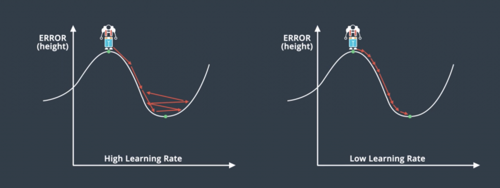
The question of what learning rate to use is pretty much a research question itself but here’s a general rule. If your learning rate is too big then you’re taking huge steps which could be fast at the beginning but you may miss the minimum and keep going which will make your model pretty chaotic. If you have a small learning rate you will make steady steps and have a better chance of arriving to your local minimum. This may make your model very slow, but in general, a good rule of thumb is if your model’s not working, decrease the learning rate. The best learning rates are those which decrease as the model is getting closer to a solution.