Introduction

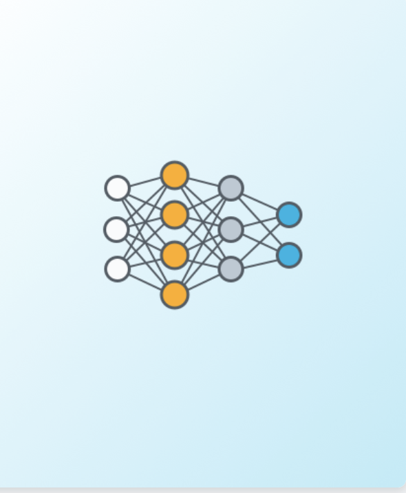
So let’s start with two questions, what is deep learning, and what is it used for? The answer to the second question is pretty much everywhere. Recent applications include things such as beating humans in games such as Go, or even jeopardy, detecting spam in emails, forecasting stock prices, recognizing images in a picture, and even diagnosing illnesses sometimes with more precision than doctors. And what is at the heart of deep learning? This wonderful object called neural networks. Neural networks vaguely mimic the process of how the brain operates, with neurons that fire bits of information. As a matter of fact, the first time I heard of a neural network, this is the image that came into my head, some scary robot with artificial brain.

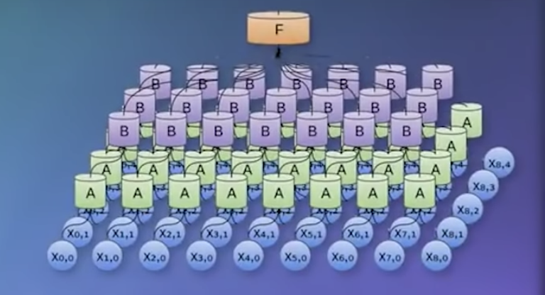
But then, I got to learn a bit more about neural networks and I realized that there are actually a lot scarier than that. his is how a neural network looks.

But after looking at neural networks for a while, I realized that they’re actually a lot simpler than that. When I think of a neural network, this is actually the image that comes to my mind.There is a child playing in the sand, with some red and blue shells and we are the child. Can you draw a line that separates the red and the blue shells? And the child draws this line. That’s it. That’s what a neural network does.

Given some data in the form of blue or red points, the neural network will look for the best line that separates them. And if the data is a bit more complicated like this one over here, then we’ll need a more complicated algorithm. Here, a deep neural network will do the job and find a more complex boundary that separates the points.

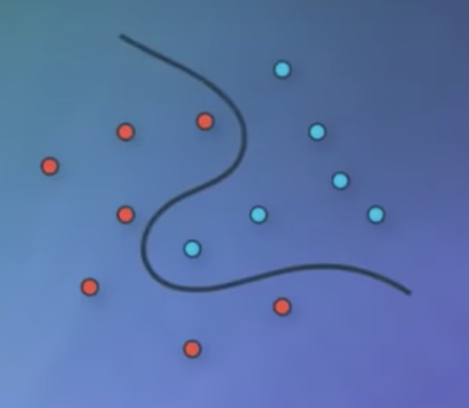
Classification Problems 1

So, let’s start with one classification example. Let’s say we are the admissions office at a university and our job is to accept or reject students. So, in order to evaluate students, we have two pieces of information, the results of a test and their grades in school. So, let’s take a look at some sample students. We’ll start with Student 1 who got 9 out of 10 in the test and 8 out of 10 in the grades. That student did quite well and got accepted. Then we have Student 2 who got 3 out of 10 in the test and 4 out of 10 in the grades, and that student got rejected. And now, we have a new Student 3 who got 7 out of 10 in the test and 6 out of 10 in the grades, and we’re wondering if the student gets accepted or not.

So, our first way to find this out is to plot students in a graph with the horizontal axis corresponding to the score on the test and the vertical axis corresponding to the grades, and the students would fit here.

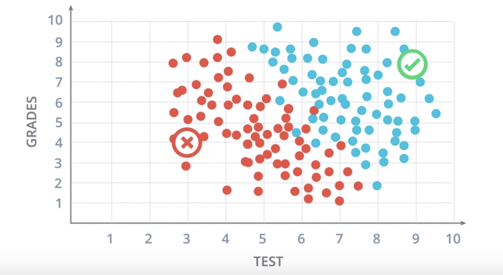
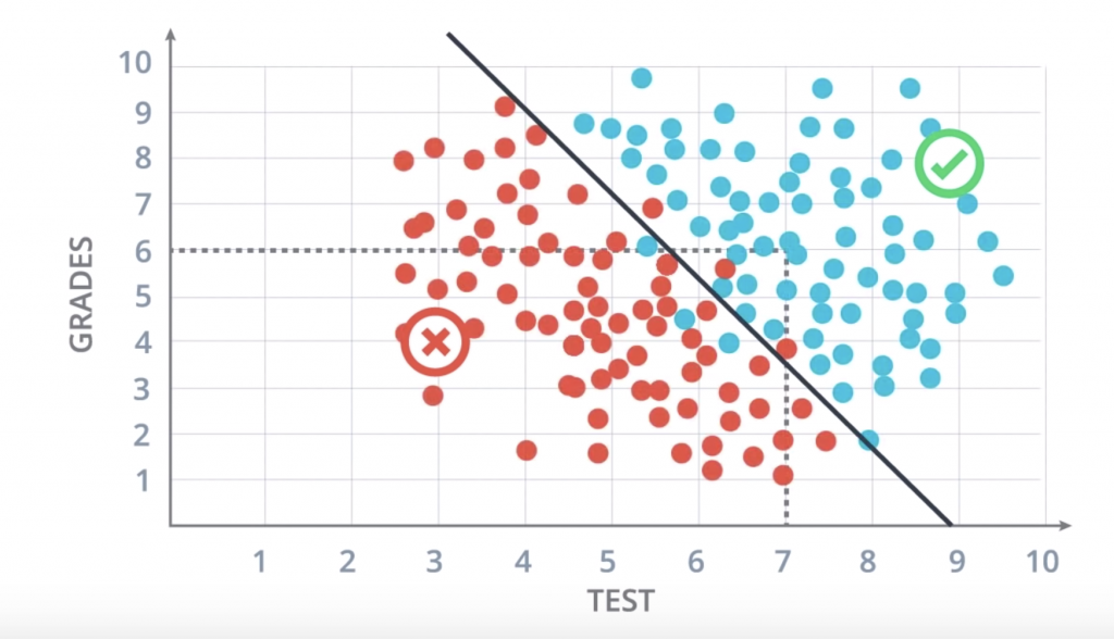
These are all the previous students who got accepted or rejected. The blue points correspond to students that got accepted, and the red points to students that got rejected. So we can see in this diagram that the students would did well in the test and grades are more likely to get accepted, and the students who did poorly in both are more likely to get rejected. does the Student 3 get accepted or rejected? you can figure it out by yourself

Classification Problems 2

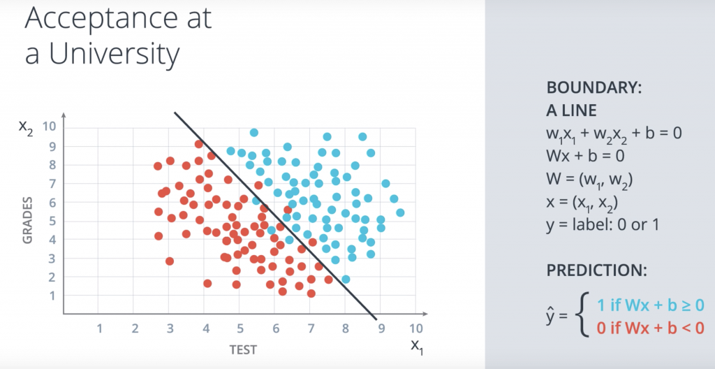
it seems that this data can be nicely separated by a line which is this line over here, and it seems that most students over the line get accepted and most students under the line get rejected. So this line is going to be our model. And now a question arises. The question is, how do we find this line?

Linear Boundaries

So, first let’s add some math. We’re going to label the horizontal axis corresponding to the test by the variable x1, and the vertical axis corresponding to the grades by the variable x2. So this boundary line that separates the blue and the red points is going to have a linear equation. The one drawn has equation 2×1+x2-18=0. What does this mean? This means that our method for accepting or rejecting students simply says the following: take this equation as our score, the score is 2xtest+grades-18. Now when the student comes in, we check their score. If their score is a positive number, then we accept the student and if the score is a negative number then we reject the student. This is called a prediction. And that’s it. That linear equation is our model.

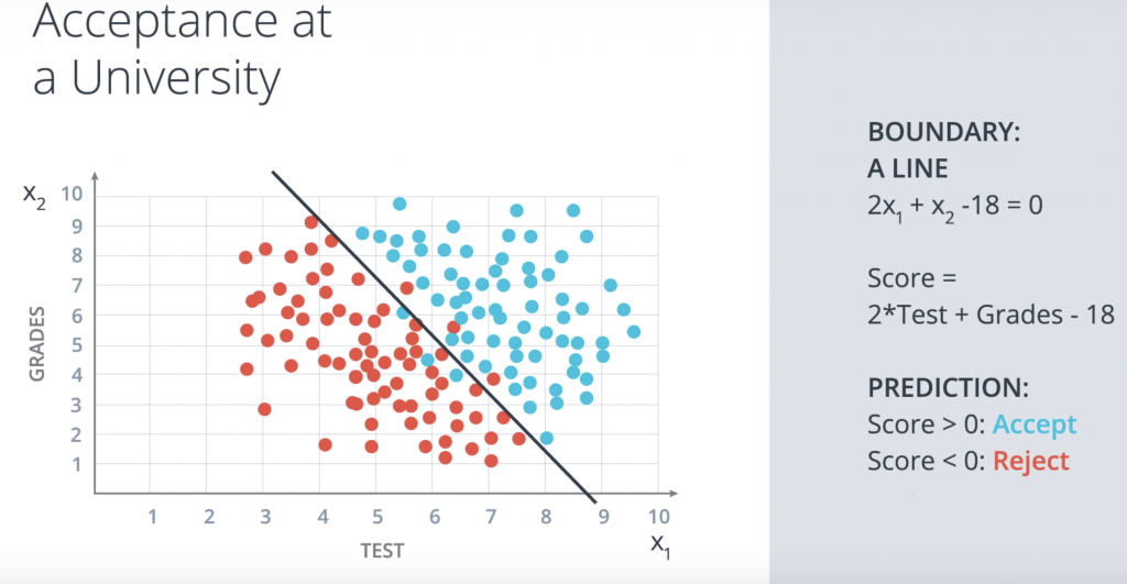
In the more general case, our boundary will be an equation of the following wx1+w2x2+b=0. We’ll abbreviate this equation in vector notation as wx+b=0, where w is the vector w1w2 and x is the vector x1x2. And we simply take the product of the two vectors. We’ll refer to x as the input, to w as the weights and b as the bias. Now, for a student coordinates x1x2, we’ll denote a label as Y and the label is what we’re trying to predict. So if the student gets accepted, namely the point is blue, then the label is 1. And if the student gets rejected, namely the point is red and then the label is 0.

Perceptrons

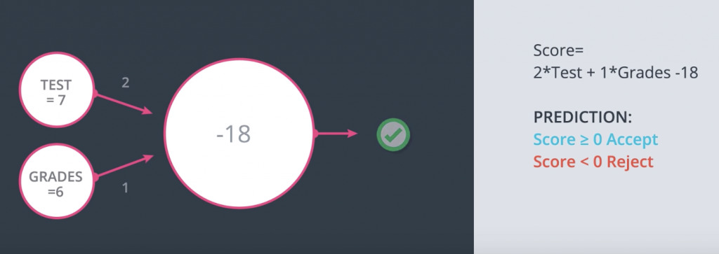
we’ll introduce the notion of a preceptron, which is the building block of neural networks, and it’s just an encoding of our equation into a small graph. The way we’ve build it is the following. Here we have our data and our boundary line and we fit it inside a node. And now we add small nodes for the inputs which, in this case, they are the test and the grades. Here we can see an example where test equals 7 and grades equals 6. And what the perceptron does is it blocks the points 7, 6 and checks if the point is in the positive or negative area. If the point is in the positive area, then it returns a yes. And if it is in the negative area, it returns a no.

Perceptron Trick

So we had a question we’re trying to answer and the question is, how do we find this line that separates the blue points from the red points in the best possible way? Let’s answer this question by first looking at a small example with three blue points and three red points. And we’re going to describe an algorithm that will find the line that splits these points properly. So the computer doesn’t know where to start. It might as well start at a random place by picking a random linear equation. This equation will define a line and a positive and negative area given in blue and red respectively.

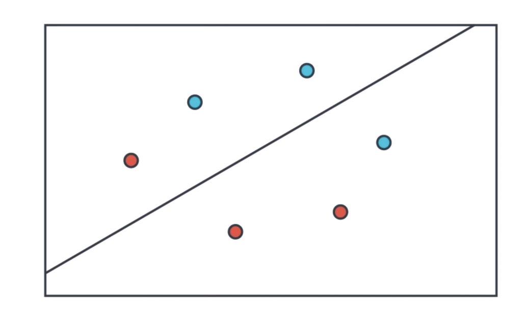
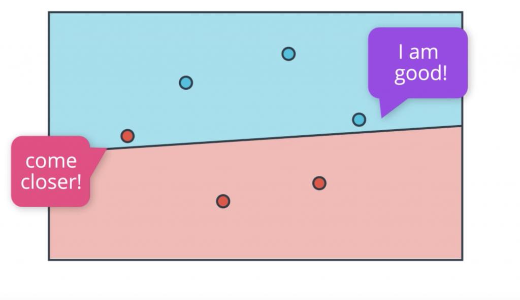
What we’re going to do is to look at how badly this line is doing and then move it around to try to get better and better. Now the question is, how do we find how badly this line is doing? So let’s ask all the points. Here we have four points that are correctly classified. They are these two blue points in the blue area and these two red points in the red area. And these points are correctly classified, so they say, “I’m good.”

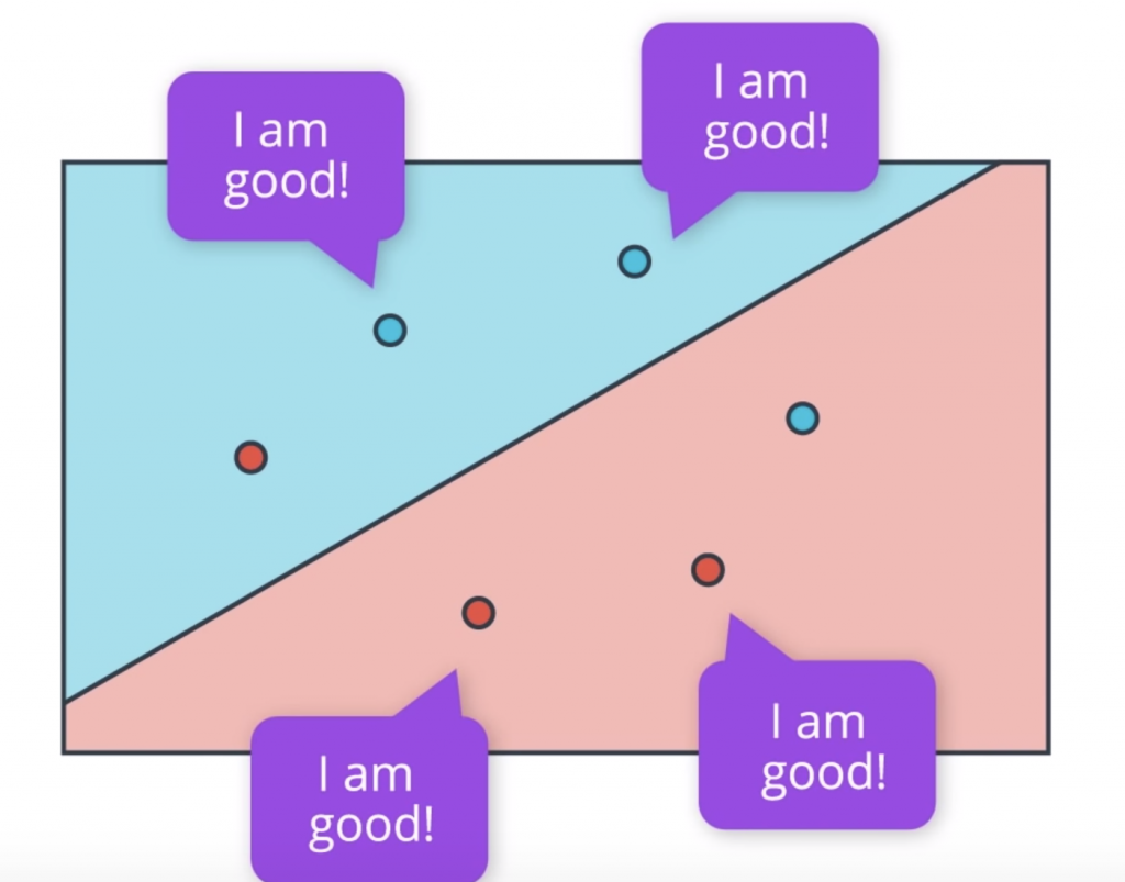
And then we have these two points that are incorrectly classified. That’s this red point in the blue area and this blue point in the red area. We want to get as much information from them so we want them to tell us something so that we can improve this line. So what is it that they can tell us?. Well, consider this. If you’re in the wrong area, you would like the line to go over you, in order to be in the right area. Thus, the points just come closer! So the line can move towards it and eventually classify it correctly.

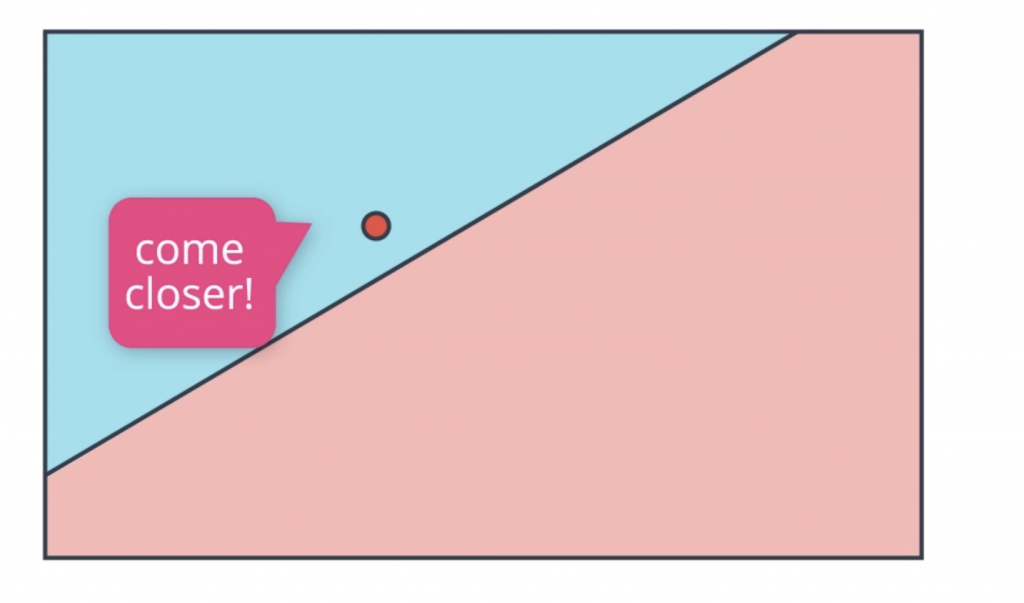
Perceptron Algorithm

Now, we finally have all the tools for describing the perceptron algorithm. We start with the random equation, which will determine some line, and two regions, the positive and the negative region. Now, we’ll move this line around to get a better and better fit. So, we ask all the points how they’re doing. The four correctly classified points say, “I’m good.” And the two incorrectly classified points say, “Come closer.”

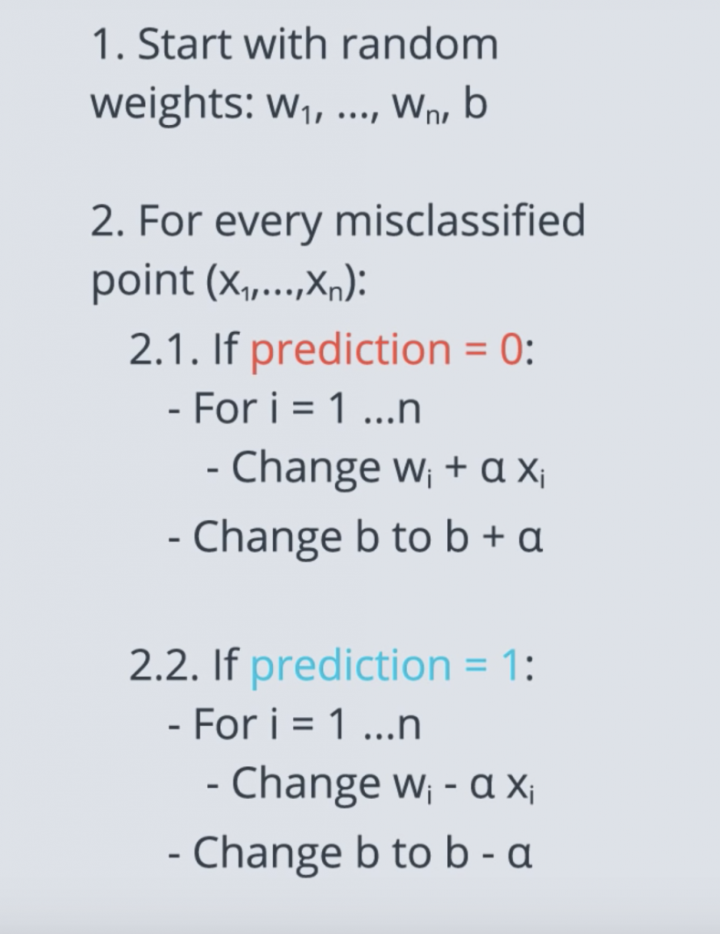
let’s actually write the pseudocode for this perceptron algorithm

Log-loss Error Function

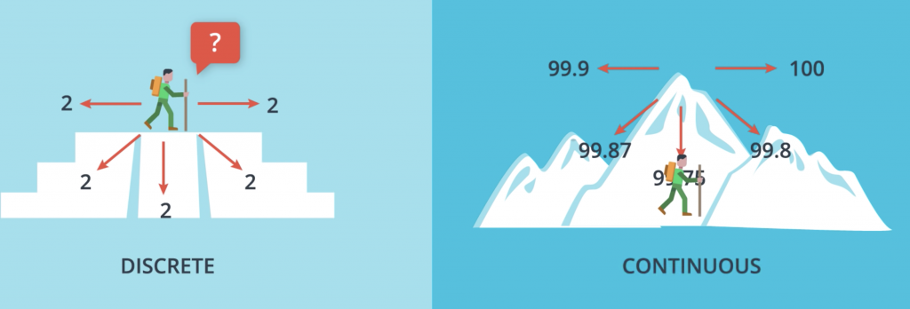
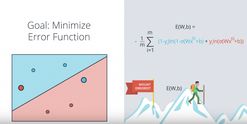
Here is obvious realization of the error function. We’re standing on top a mountain, Mount “Errorest” and I want to descend but it’s not that easy because it’s cloudy and the mountain is very big, so we can’t really see the big picture. What we’ll do to go down is we’ll look around us and we consider all the possible directions in which we can walk. Then we pick a direction that makes us descend the most. Let’s say it’s this one over here. So we take a step in that direction. Thus, we’ve decreased the height. Once we take the step and we start the process again and again always decreasing the height until we go all the way down the mountain, minimizing the height. In this case the key metric that we use to solve the problem is the height.

There’s a small problem with this approach. In our algorithms we’ll be taking very small steps and the reason for that is calculus, because our tiny steps will be calculated by derivatives. So what happens if we take very small steps here? We start with two errors and then move a tiny amount and we’re still at two errors. Then move a tiny amount again and we’re still two errors. Another tiny amount and we’re still at two and again and again. So not much we can do here. This is equivalent to using gradient descent to try to descend from an Aztec pyramid with flat steps. If we’re standing here in the second floor, for the two errors and we look around ourselves, we’ll always see two errors and we’ll get confused and not know what to do. On the other hand in Errorest we can detect very small variations in height and we can figure out in what direction it can decrease the most. In math terms this means that in order for us to do gradient descent our error function can not be discrete, it should be continuous.

Softmax

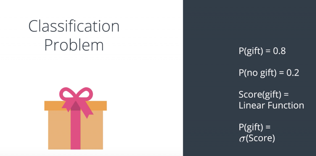
Let’s switch to a different example for a moment. Let’s say we have a model that will predict if you receive a gift or not. So, the model use predictions in the following way. It says, the probability that you get a gift is 0.8, which automatically implies that the probability that you don’t receive a gift is 0.2. And what does the model do? What the model does is take some inputs. For example, is it your birthday or have it been good all year? And based on those inputs, it calculates a linear model which would be the score. Then, the probability that you get the gift or not is simply the sigmoid function applied to that score.

Now, what if you had more options than just getting a gift or not a gift? Let’s say we have a model that just tell us what animal we just saw, and the options are a duck, a beaver and a walrus. We want a model that tells an answer along the lines of the probability of a duck is 0.67, the probability of a beaver is 0.24, and the probability of a walrus is 0.09. Notice that the probabilities need to add to one.

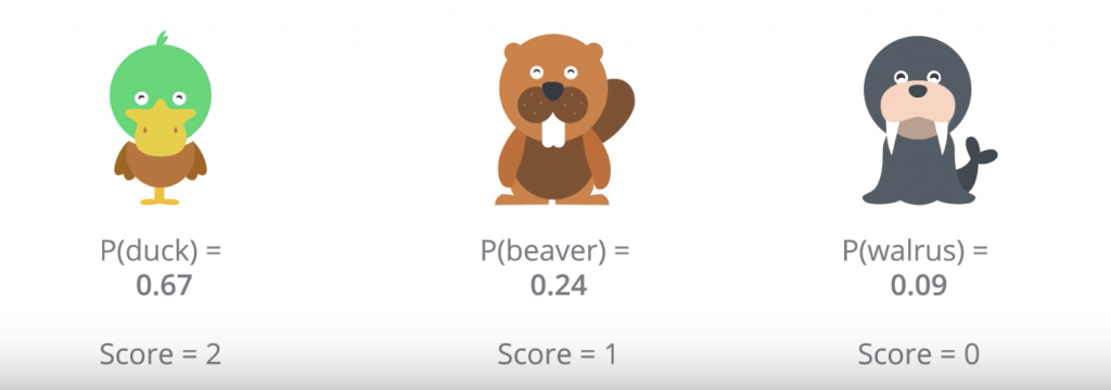
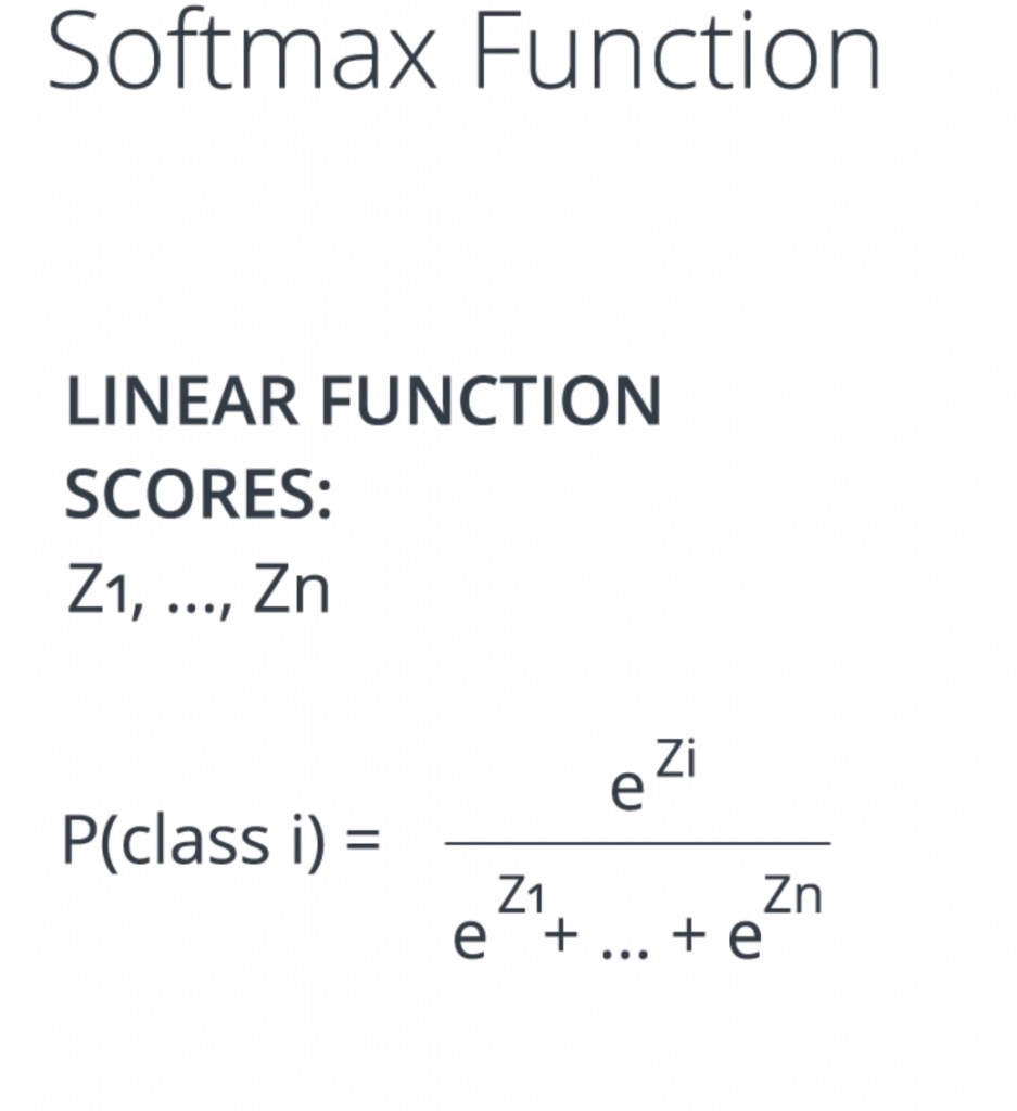
Let’s say we have a linear model based on some inputs. The inputs could be, does it have a beak or not? Number of teeth. Number of feathers. Hair, no hair. Does it live in the water? Does it fly? Etc. We calculate linear function based on those inputs, and let’s say we get some scores. So, the duck gets a score of two, and the beaver gets a score of one, and the walrus gets a score of zero. And now the question is, how do we turn these scores into probabilities? we take the exponential of each score; divide each exponential score to the sum of all exponential socre

One-Hot Encoding

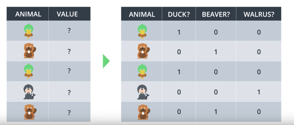
let’s say, our classes are Duck, Beaver and Walrus? What variable do we input in the algorithm? Maybe, we can input a 0 or 1 and a 2, but that would not work because it would assume dependencies between the classes that we can’t have. So, this is what we do. What we do is, we come up with one variable for each of the classes. So, our table becomes like this.

Maximum Likelihood

So we’re still in our quest for an algorithm that will help us pick the best model that separates our data. Well, since we’re dealing with probabilities then let’s use them in our favor. Let’s say I’m a student and I have two models. One that tells me that my probability of getting accepted is 80% and one that tells me the probability is 55%. Which model looks more accurate? Well, if I got accepted then I’d say the better model is probably the one that says 80%. What if I didn’t get accepted? Then the more accurate model is more likely the one that says 55 percent. So let me be more specific. Let’s look at the following four points: two blue and two red and two models that classify them, the one on the left and the one on the right. Quick. Which model looks better?

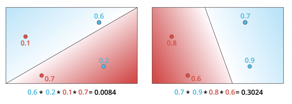
The model on the right is much better since it classifies the four points correctly whereas the model in the left gets two points correctly and two points incorrectly. But let’s see why the model in the right is better from the probability perspective. And by that, we’ll show you that the arrangement in the right is much more likely to happen than the one in the left. So let’s recall that our prediction is ŷ = σ(Wx+b) and that is precisely the probability of a point being labeled positive which means blue. So for the points in the figure, let’s say the model tells you that the probability of being blue are 0.9, 0.6, 0.3, and 0.2. Notice that the points in the blue region are much more likely to be blue and the points in the red region are much less likely to be blue. Now if we assume that the colors of the points are independent events then the probability for the whole arrangement is the product of the probabilities of the four points. As we saw the model on the left tells us that the probabilities of these points being of those colors is 0.0084. If we do the same thing for the model on the right. Let’s say we get that the probabilities of the two points in the right being blue are 0.7 and 0.9 and of the two points in the left being red are 0.8 and 0.6. When we multiply these we get 0.3024 which is around 30%. This is much higher than 0.0084. Thus, we confirm that the model on the right is better because it makes the arrangement of the points much more likely to have those colors. So now, what we do is the following? We start from the bad modeling, calculate the probability that the points are those colors, multiply them and we obtain the total probability is 0.0084. Now if we just had a way to maximize this probability we can increase it all the way to 0.3024. Thus, our new goal becomes precisely that, to maximize this probability. This method, as we stated before, is called maximum likelihood.

Maximizing Probabilities

Well we’re getting somewhere now. We’ve concluded that the probability is important. And that the better model will give us a better probability. Now the question is, how we maximize the probability. Also, if remember correctly we’re talking about an error function and how minimizing this error function will take us to the best possible solution. Could these two things be connected? Could we obtain an error function from the probability? Could it be that maximizing the probability is equivalent to minimizing the error function? Maybe. So a quick recap. We have two models, the bad one on the left and the good one on the right.

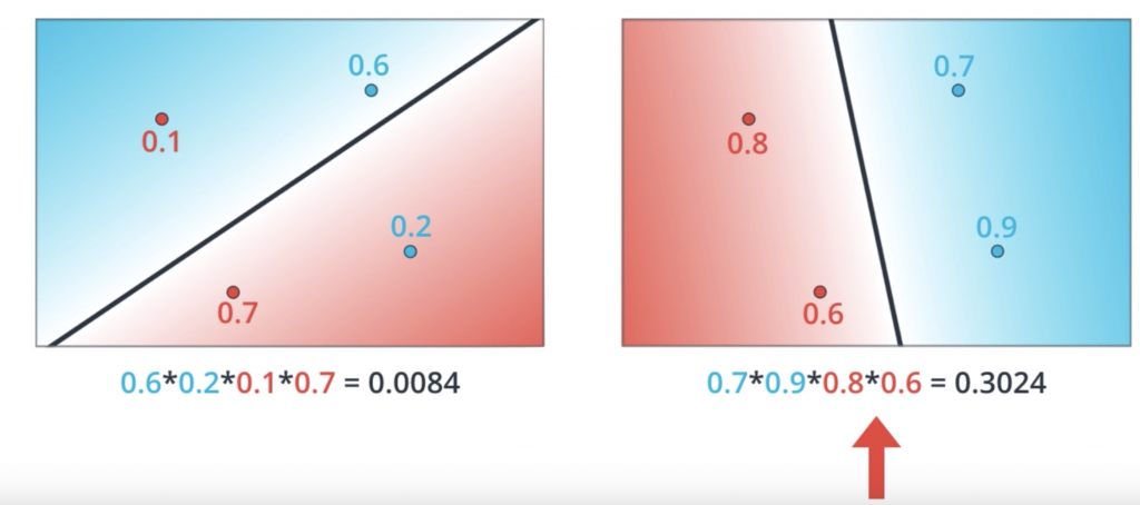
And the way to tell they’re bad or good is to calculate the probability of each point being the color it is according to the model. Multiply these probabilities in order to obtain the probability of the whole arrangement and then check that the model on the right gives us a much higher probability than the model on the left. Now all we need to do is to maximize this probability. But probability is a product of numbers and products are hard. Maybe this product of four numbers doesn’t look so scary. But what if we have thousands of datapoints? That would correspond to a product of thousands of numbers, all of them between zero and one. This product would be very tiny, something like 0.0000 something and we definitely want to stay away from those numbers. Also, if I have a product of thousands of numbers and I change one of them, the product will change drastically. In summary, we really want to stay away from products. And what’s better than products? it’s sum

Cross-Entropy

logarithm has this very nice identity that says that the logarithm of the product A times B is the sum of the logarithms of A and B. So this is what we do. We take our products and we take the logarithms, so now we get a sum of the logarithms of the factors. So the ln(0.60.20.1*0.7) is equal to ln(0.6) + ln(0.2) + ln(0.1) + ln(0.7) etc

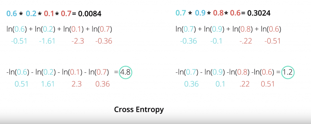
We can calculate those values and get minus 0.51, minus 1.61, minus 0.23 etc. Notice that they are all negative numbers and that actually makes sense. This is because the logarithm of a number between 0 and 1 is always a negative number since the logarithm of one is zero. So it actually makes sense to think of the negative of the logarithm of the probabilities and we’ll get positive numbers. So that’s what we’ll do. We’ll take the negative of the logarithm of the probabilities. That sums up negatives of logarithms of the probabilities, we’ll call the cross entropy

Let’s look a bit closer into Cross-Entropy by switching to a different example. Let’s say we have three doors. And no this is not the Monty Hall problem. We have the green door, the red door, and the blue door, and behind each door we could have a gift or not have a gift. And the probabilities of there being a gift behind each door is 0.8 for the first one, 0.7 for the second one, 0.1 for the third one. So for example behind the green door there is an 80 percent probability of there being a gift, and a 20 percent probability of there not being a gift. So we can put the information in this table where the probabilities of there being a gift are given in the top row, and the probabilities of there not being a gift are given in the bottom row. So let’s say we want to make a bet on the outcomes. So we want to try to figure out what is the most likely scenario here. And for that we’ll assume they’re independent events. In this case, the most likely scenario is just obtained by picking the largest probability in each column. So for the first door is more likely to have a gift than not have a gift. So we’ll say there’s a gift behind the first door. For the second door, it’s also more likely that there’s a gift. So we’ll say there’s a gift behind the second door. And for the third door it’s much more likely that there’s no gift, so we’ll say there’s no gift behind the third door. And as the events are independent, the probability for this whole arrangement is the product of the three probabilities which is 0.8, times 0.7, times 0.9, which ends up being 0.504, which is roughly 50 percent.

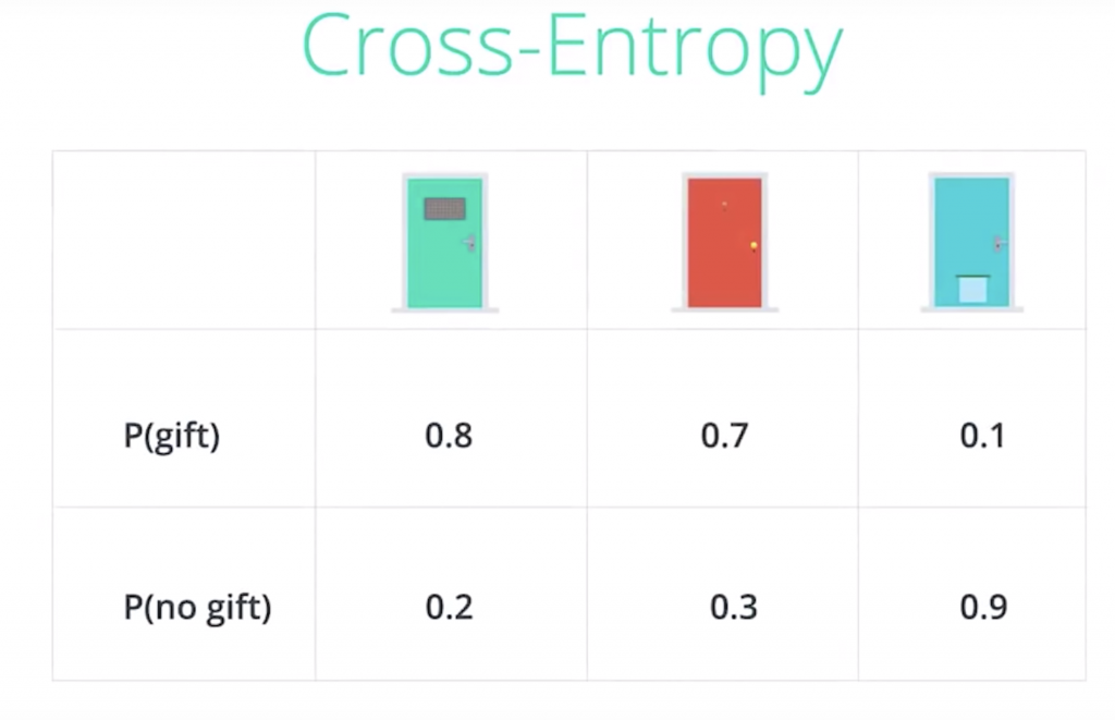
we learned that the negative of the logarithm of the probabilities across entropy. So let’s go ahead and calculate the cross-entropy. And notice that the events with high probability have low cross-entropy and the events with low probability have high cross-entropy. For example, the second row which has probability of 0.504 gives a small cross-entropy of 0.69, and the second to last row which is very very unlikely has a probability of 0.006 gives a cross entropy a 5.12.

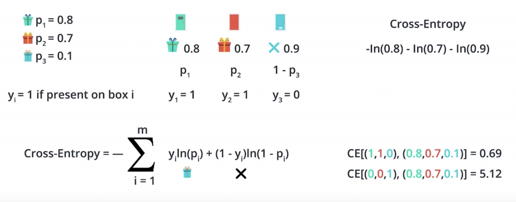
So when we calculate the cross-entropy, we get the negative of the logarithm of the product, which is a sum of the negatives of the logarithms of the factors. Now that was when we had two classes namely receiving a gift or not receiving a gift. What happens if we have more classes? Let’s take a look. So we have a similar problem. We still have three doors. And this problem is still not the Monty Hall problem. Behind each door there can be an animal, and the animal can be of three types. It can be a duck, it can be a beaver, or it can be a walrus. So let’s look at this table of probabilities.

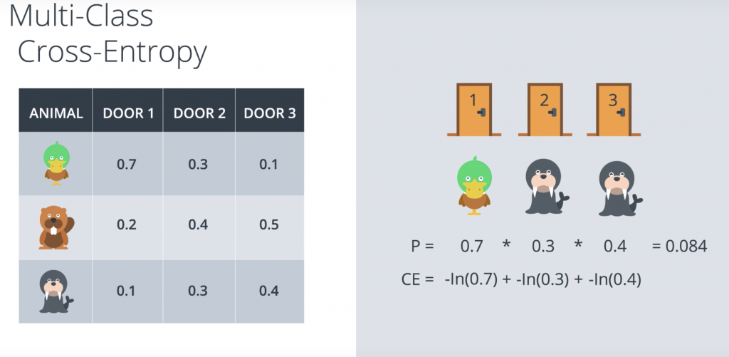
So let’s look at a sample scenario. Let’s say we have our three doors, and behind the first door, there’s a duck, behind the second door there’s a walrus, and behind the third door there’s also a walrus. Recall that the probabilities are again by the table. So a duck behind the first door is 0.7 likely, a walrus behind the second door is 0.3 likely, and a walrus behind the third door is 0.4 likely. So the probability of obtaining this three animals is the product of the probabilities of the three events since they are independent events, which in this case it’s 0.084. And as we learn, that cross entropy here is given by the sums of the negatives of the logarithms of the probabilities. The Cross entropy’s and the sum of these three which is actually 2.48. But we want a formula, so let’s put some variables here.

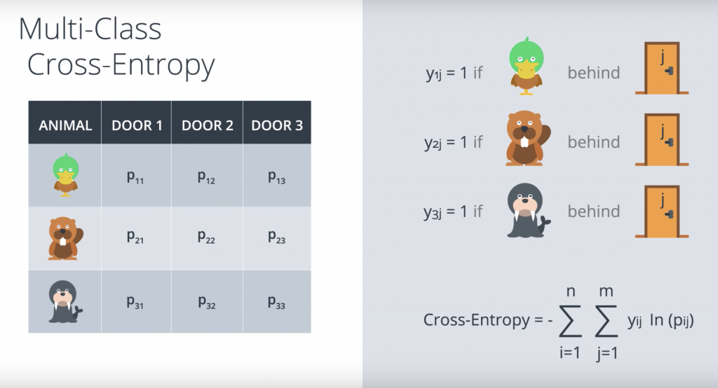
So P11 is the probability of finding a duck behind door one. P12 is the probability of finding a duck behind door two etc. And let’s have the indicator variables Y1j if there’s a duck behind door J. Y2j if there’s a beaver behind door J, and Y3j if there’s a walrus behind door J. And these variables are zero otherwise. And so, the formula for the cross entropy is as show in the previous picture

Logistic Regression

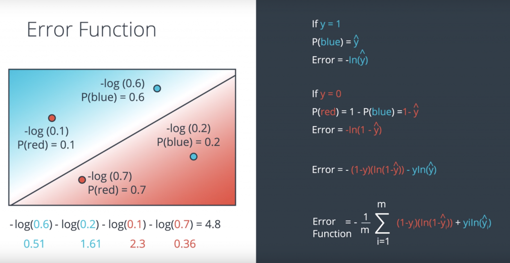
So this is a good time for a quick recap of the last couple of lessons. Here we have two models. The bad model on the left and the good model on the right. And for each one of those we calculate the cross entropy which is the sum of the negatives of the logarithms off the probabilities of the points being their colors. And we conclude that the one on the right is better because a cross entropy is much smaller. So let’s actually calculate the formula for the error function. Let’s split into two cases. The first case being when y=1. So when the point is blue to begin with, the model tells us that the probability of being blue is the prediction y_hat. So for these two points the probabilities are 0.6 and 0.2. As we can see the point in the blue area has more probability of being blue than the point in the red area. And our error is simply the negative logarithm of this probability. So it’s precisely minus logarithm of y_hat. In the figure it’s minus logarithm of 0.6. and minus logarithm of 0.2. Now if y=0, so when the point is red, then we need to calculate the probability of the point being red. The probability of the point being red is one minus the probability of the point being blue which is precisely 1 minus the prediction y_hat. So the error is precisely the negative logarithm of this probability which is negative logarithm of 1 – y_hat. We can summarize these two formulas into this one. Error = – (1-y)(ln( 1- y_hat)) – y ln(y_hat).

So now our goal is to minimize the error function and we’ll do it as follows. We started some random weights, which will give us the predictions σ(Wx+b). As we saw, that also gives us a error function given by this formula. Remember that the summands are also error functions for each point. So each point will give us a larger function if it’s mis-classified and a smaller one if it’s correctly classified. And the way we’re going to minimize this function, is to use gradient decent. So here’s Errorest and this is us, and we’re going to try to jiggle the line around to see how we can decrease the error function. Now, the error function is the height which is E(W,b) where W and b are the weights. Now what we’ll do, is we’ll use gradient decent in order to get to the bottom of the mountain at a much smaller height, which gives us a smaller error function E of W’, b’.

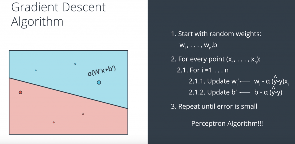
Gradient Descent

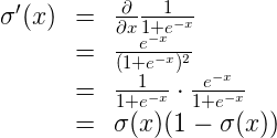
In the last few videos, we learned that in order to minimize the error function, we need to take some derivatives. So let’s get our hands dirty and actually compute the derivative of the error function. The first thing to notice is that the sigmoid function has a really nice derivative. Namely,

The reason for this is the following, we can calculate it using the quotient formula:

 the error formula is:

where the prediction is given by

Our goal is to calculate the gradient of E at a point x=(x1​,…,xn​), given by the partial derivatives

To simplify our calculations, we’ll actually think of the error that each point produces, and calculate the derivative of this error. The total error, then, is the average of the errors at all the points. The error produced by each point is, simply

in order to calculate the derivative of this error with respect to the weights, we’ll first calculate

Now, we can go ahead and calculate the derivative of the error E at a point x

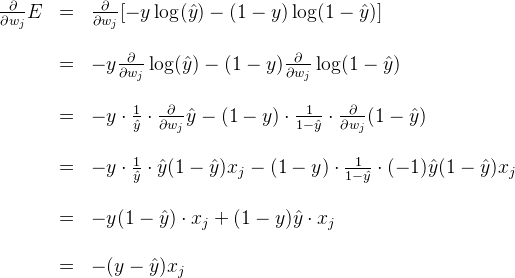
A similar calculation will show us that

Therefore, since the gradient descent step simply consists in subtracting a multiple of the gradient of the error function at every point, then this updates the weights in the following way:

which is equivalent to

Similarly, it updates the bias in the following way:

Non-linear Data

Now we’ve been dealing a lot with data sets that can be separated by a line, But as you can imagine the real world is much more complex than that. This is where neural networks can show their full potential. So, let’s go back to this example of where we saw some data that is not linearly separable.

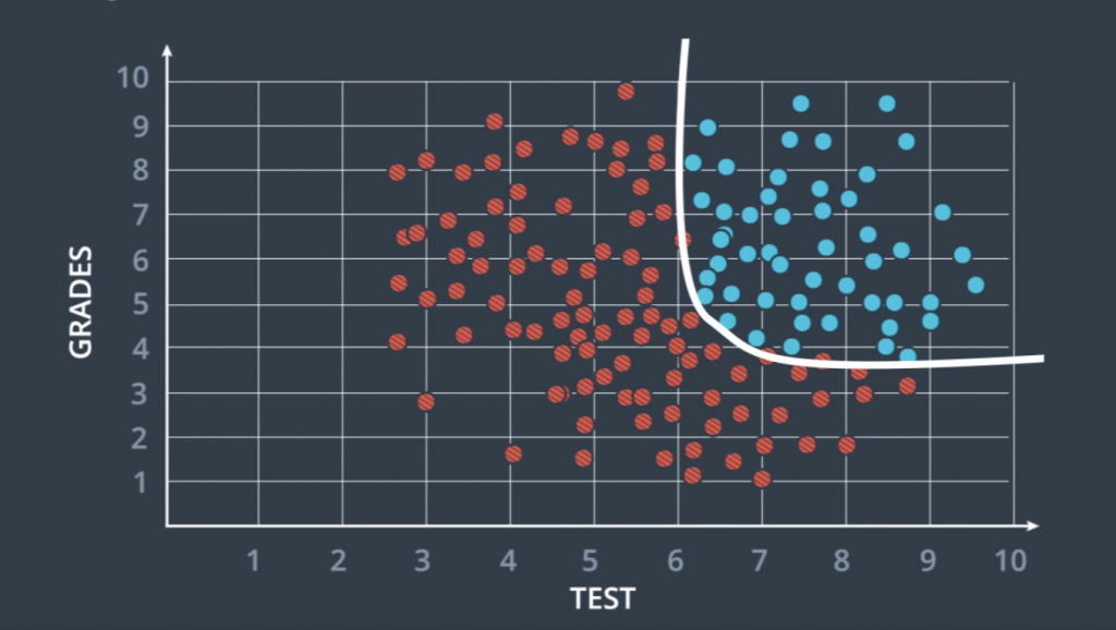
So a line can not divide these red and blue points and we looked at some solutions, and if you remember, the one we considered more seriously was this curve over here. So what I’ll teach you now is to find this curve and it’s very similar than before. We’ll still use grading dissent. In a nutshell, what we’re going to do is for these data which is not separable with a line, we’re going to create a probability function where the points in the blue region are more likely to be blue and the points in the red region are more likely to be red. And this curve here that separates them is a set of points which are equally likely to be blue or red. Everything will be the same as before except this equation won’t be linear and that’s where neural networks come into play.

Neural Network Architecture

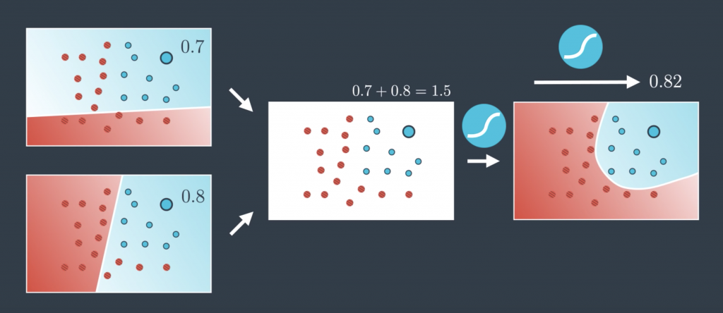
Now I’m going to show you how to create these nonlinear models. What we’re going to do is a very simple trick. We’re going to combine two linear models into a nonlinear model as follows. Visually it looks like this. The two models over imposed creating the model on the right. It’s almost like we’re doing arithmetic on models. It’s like saying “This line plus this line equals that curve.” Let me show you how to do this mathematically. So a linear model as we know is a whole probability space. This means that for every point it gives us the probability of the point being blue. So, for example, this point over here is in the blue region so its probability of being blue is 0.7. The same point given by the second probability space is also in the blue region so it’s probability of being blue is 0.8. Now the question is, how do we combine these two? Well, the simplest way to combine two numbers is to add them, right? So 0.8 plus 0.7 is 1.5. But now, this doesn’t look like a probability anymore since it’s bigger than one. And probabilities need to be between 0 and 1. So what can we do? How do we turn this number that is larger than 1 into something between 0 and 1? Well, we’ve been in this situation before and we have a pretty good tool that turns every number into something between 0 and 1. That’s just a sigmoid function. So that’s what we’re going to do. We applied the sigmoid function to 1.5 to get the value 0.82 and that’s the probability of this point being blue in the resulting probability space.

Neural networks have a certain special architecture with layers. The first layer is called the input layer, which contains the inputs, in this case, x1 and x2. The next layer is called the hidden layer, which is a set of linear models created with this first input layer. And then the final layer is called the output layer, where the linear models get combined to obtain a nonlinear model.

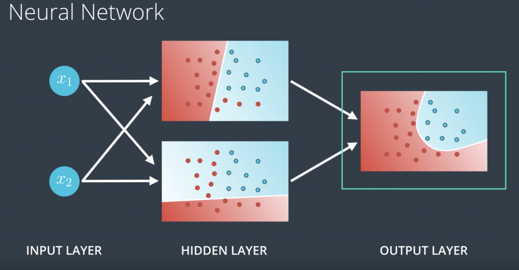
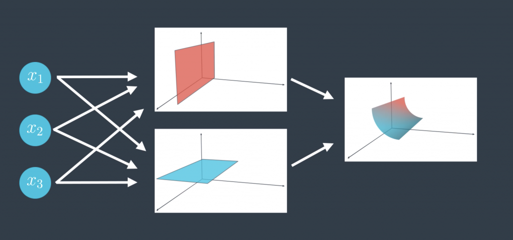
You can have different architectures. For example, here’s one with a larger hidden layer. Now we’re combining three linear models to obtain the triangular boundary in the output layer. Now what happens if the input layer has more nodes? For example, this neural network has three nodes in its input layer. Well, that just means we’re not living in two-dimensional space anymore. We’re living in three-dimensional space, and now our hidden layer, the one with the linear models, just gives us a bunch of planes in three space, and the output layer bounds a nonlinear region in three space.

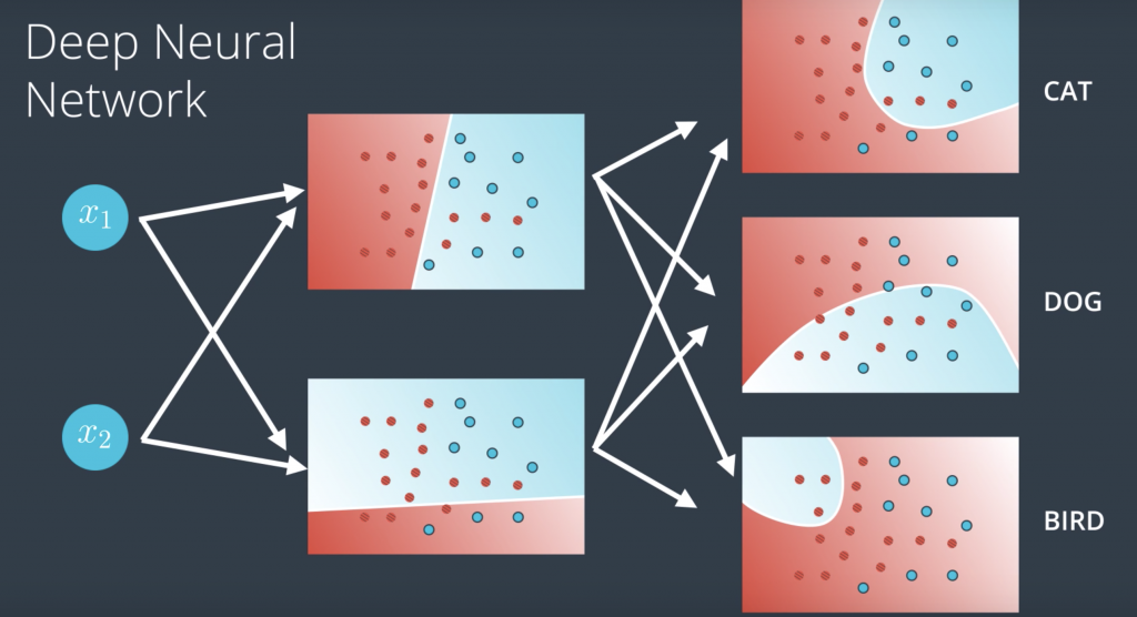
So if our model is telling us if an image is a cat or dog or a bird, then we simply have each node in the output layer output a score for each one of the classes: one for the cat, one for the dog, and one for the bird. And finally, and here’s where things get pretty cool, what if we have more layers? Then we have what’s called a deep neural network. Now what happens here is our linear models combine to create nonlinear models and then these combine to create even more nonlinear models. In general, we can do this many times and obtain highly complex models with lots of hidden layers. This is where the magic of neural networks happens.

Feedforward

So now that we have defined what neural networks are, we need to learn how to train them. Training them really means what parameters should they have on the edges in order to model our data well. So in order to learn how to train them, we need to look carefully at how they process the input to obtain an output. Now the perceptron is defined by a linear equation say w1, x1 plus w2, x2 plus B, where w1 and w2 are the weights in the edges and B is the bias in the note. Here, w1 is bigger than w2, so we’ll denote that by drawing the edge labelled w1 much thicker than the edge labelled w2. Now, what the perceptron does is it plots the point x1, x2 and it outputs the probability that the point is blue. Here is the point is in the red area and then the output is a small number, since the point is not very likely to be blue. This process is known as feedforward.

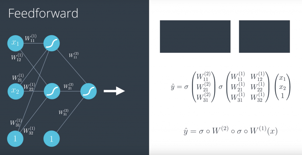
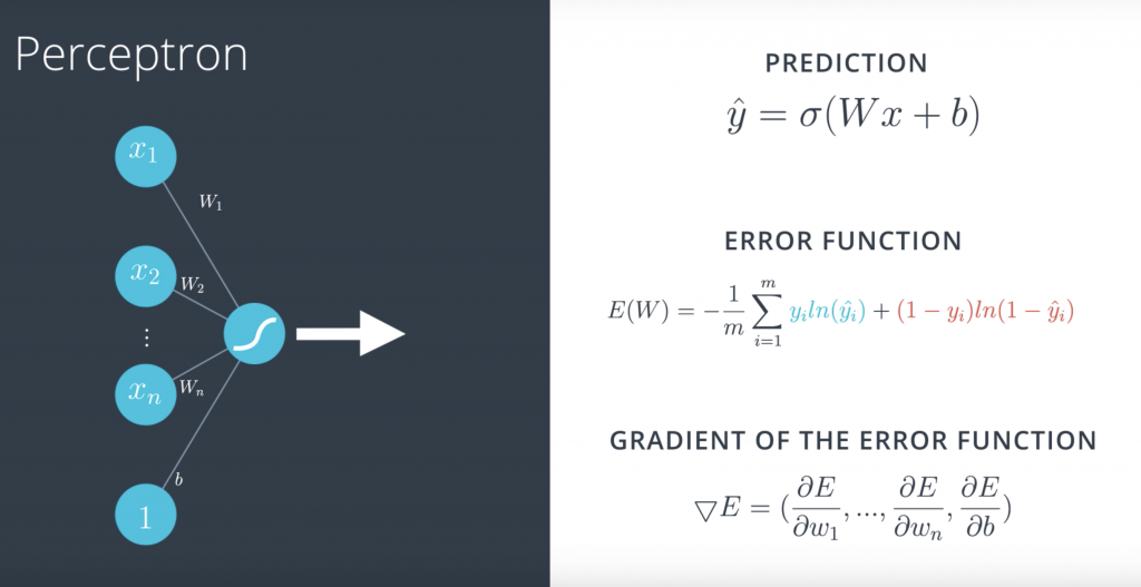
So, our goal is to train our neural network. In order to do this, we have to define the error function. So, let’s look again at what the error function was for perceptrons. So, here’s our perceptron. In the left, we have our input vector with entries x_1 up to x_n, and one for the bias unit. And the edges with weights W_1 up to W_n, and b for the bias unit. Finally, we can see that this perceptron uses a sigmoid function. And the prediction is defined as y-hat equals sigmoid of Wx plus b. And as we saw, this function gives us a measure of the error of how badly each point is being classified.

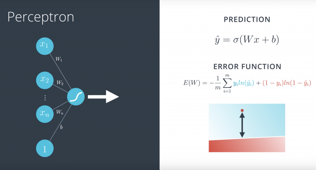
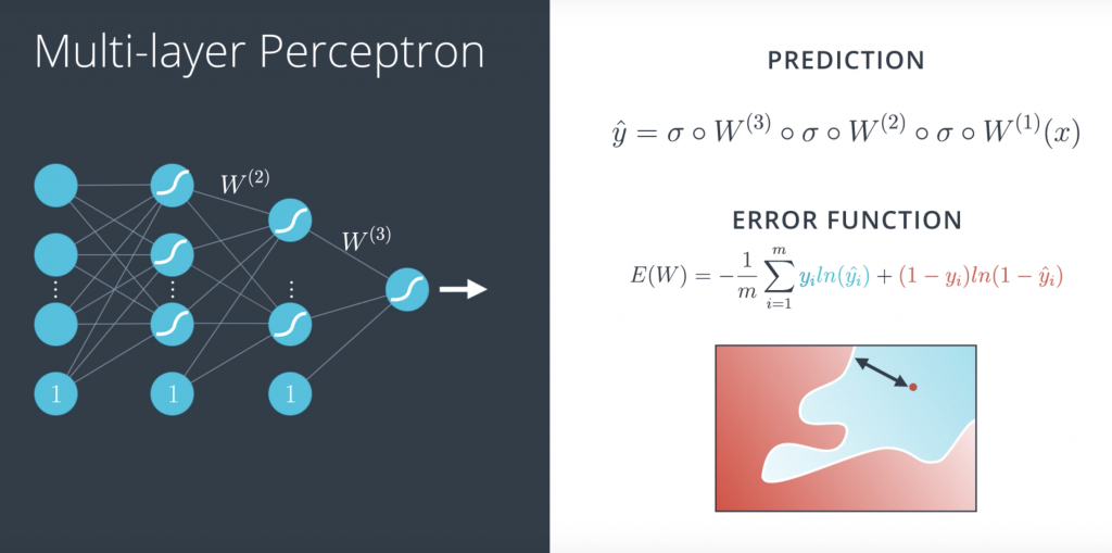
So, what are we going to do to define the error function in a multilayer perceptron? Well, as we saw, our prediction is simply a combination of matrix multiplications and sigmoid functions.But the error function can be the exact same thing, right? It can be the exact same formula

Backpropagation

On your left, you have a single perceptron with the input vector, the weights and the bias and the sigmoid function inside the node. And on the right, we have a formula for the prediction, which is the sigmoid function of the linear function of the input. And below, we have a formula for the error, which is the average of all points of the blue term for the blue points and the red term for the red points. And in order to descend from Errorest, we calculate the gradient. And the gradient is simply the vector formed by all the partial derivatives of the error function with respect to the weights w1 up to wn and and the bias b

and what do we do in a multilayer perceptron? Well, this time it’s a little more complicated but it’s pretty much the same thing

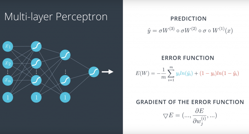
If we want to write this more formally, we recall that the prediction is a composition of sigmoids and matrix multiplications, where these are the matrices and the gradient is just going to be formed by all these partial derivatives. Here, it looks like a matrix but in reality it’s just a long vector. And the gradient descent is going to do the following;

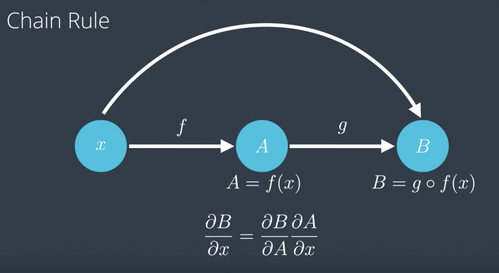
So before we start calculating derivatives, let’s do a refresher on the chain rule which is the main technique we’ll use to calculate them. The chain rule says, if you have a variable x on a function f that you apply to x to get f of x, which we’re gonna call A, and then another function g, which you apply to f of x to get g of f of x, which we’re gonna call B, the chain rule says, if you want to find the partial derivative of B with respect to x, that’s just a partial derivative of B with respect to A times the partial derivative of A with respect to x

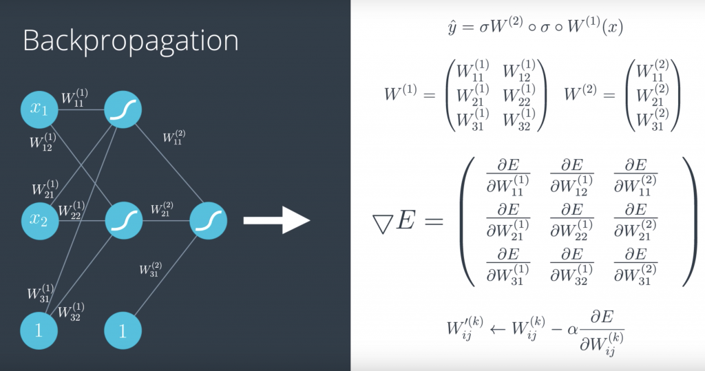
So, let us go back to our neural network with our weights and our input. And recall that the weights with superscript 1 belong to the first layer, and the weights with superscript 2 belong to the second layer. so that we can have everything in matrix notation.

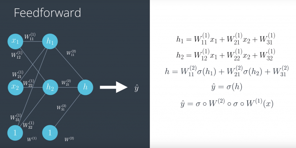
And now what happens with the input? So, let us do the feedforward process. In the first layer, we take the input and multiply it by the weights and that gives us h1, which is a linear function of the input and the weights. Same thing with h2, given by this formula over here. Now, in the second layer, we would take this h1 and h2 and the new bias, apply the sigmoid function, and then apply a linear function to them by multiplying them by the weights and adding them to get a value of h. And finally, in the third layer, we just take a sigmoid function of h to get our prediction or probability between 0 and 1, which is ŷ.

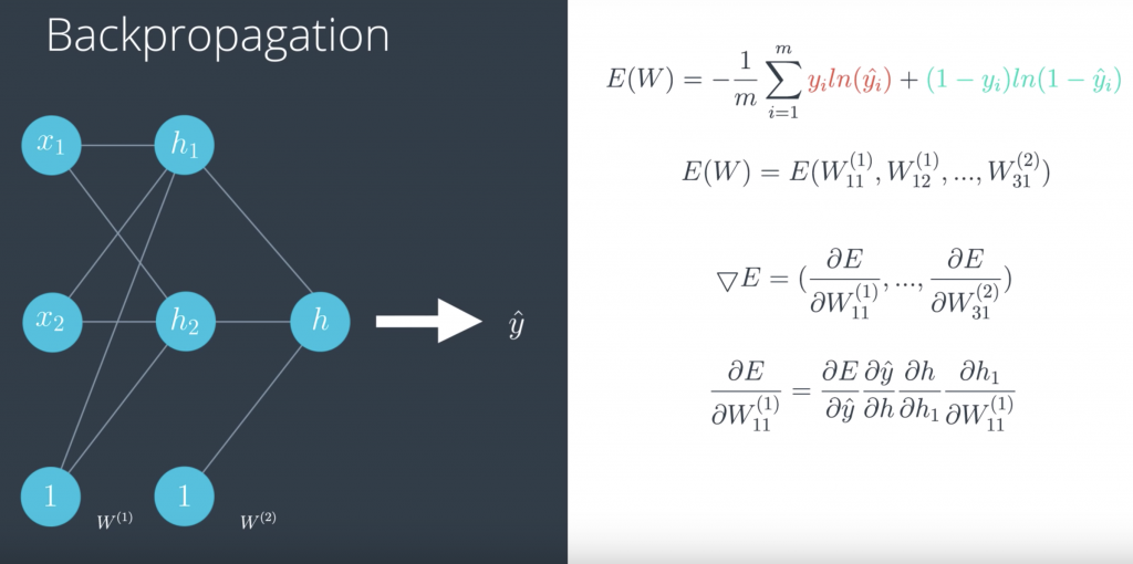
Now, we are going to develop backpropagation, which is precisely the reverse of feedforward. So, we are going to calculate the derivative of this error function with respect to each of the weights in the labels by using the chain rule. So, let us recall that our error function is this formula over here, which is a function of the prediction ŷ. But, since the prediction is a function of all the weights wij, then the error function can be seen as the function on all the wij. Therefore, the gradient is simply the vector formed by all the partial derivatives of the error function E with respect to each of the weights. So, let us calculate one of these derivatives.

Lab

we have hand-on lab & assignment take a look at our jupyter server at
http://14.232.166.121:8880/lab? > deeplearning/intro-neural-networks