Gradient Descent with Squared Errors

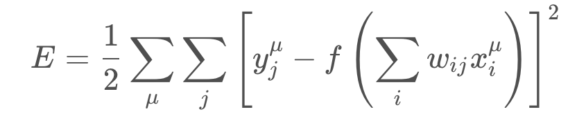
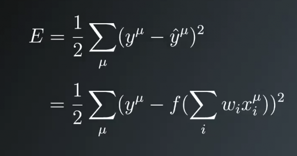
We want to find the weights for our neural networks. Let’s start by thinking about the goal. The network needs to make predictions as close as possible to the real values. To measure this, we use a metric of how wrong the predictions are, the error. A common metric is the sum of the squared errors (SSE):

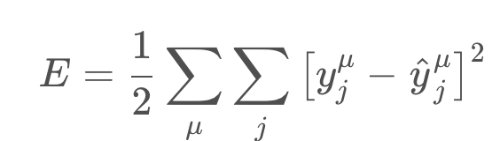
where y^​ is the prediction and y is the true value, and you take the sum over all output units j and another sum over all data points μ. This might seem like a really complicated equation at first, but it’s fairly simple once you understand the symbols and can say what’s going on in words.

First, the inside sum over j. This variable j represents the output units of the network. So this inside sum is saying for each output unit, find the difference between the true value y and the predicted value from the network y^​, then square the difference, then sum up all those squares.

Then the other sum over μ is a sum over all the data points. So, for each data point you calculate the inner sum of the squared differences for each output unit. Then you sum up those squared differences for each data point. That gives you the overall error for all the output predictions for all the data points.

The SSE is a good choice for a few reasons. The square ensures the error is always positive and larger errors are penalized more than smaller errors. Also, it makes the math nice, always a plus.

Remember that the output of a neural network, the prediction, depends on the weights

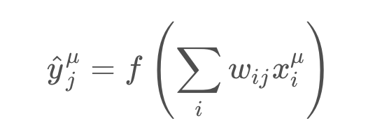
and accordingly the error depends on the weights

We want the network’s prediction error to be as small as possible and the weights are the knobs we can use to make that happen. Our goal is to find weights wij​ that minimize the squared error EE. To do this with a neural network, typically you’d use gradient descent.

Enter Gradient Descent

with gradient descent, we take multiple small steps towards our goal. In this case, we want to change the weights in steps that reduce the error. Continuing the analogy, the error is our mountain and we want to get to the bottom. Since the fastest way down a mountain is in the steepest direction, the steps taken should be in the direction that minimizes the error the most. We can find this direction by calculating the gradient of the squared error.

Gradient is another term for rate of change or slope. If you need to brush up on this concept, check out Khan Academy’s great lectures on the topic.

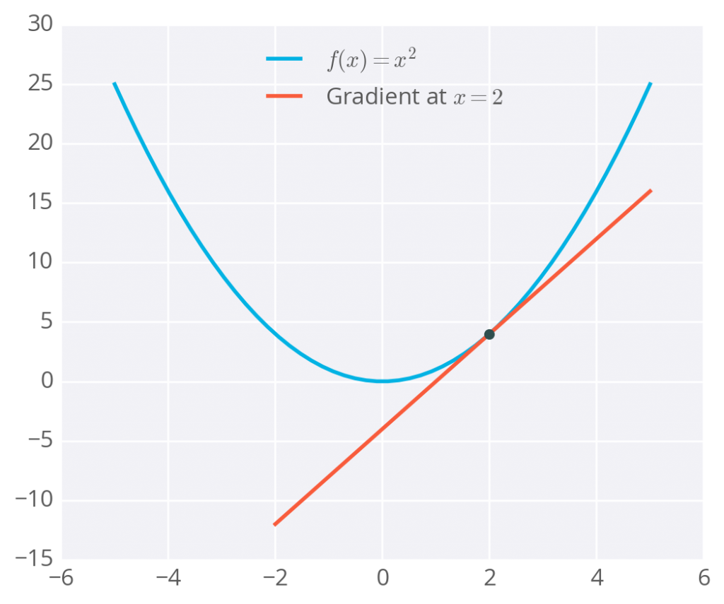
To calculate a rate of change, we turn to calculus, specifically derivatives. A derivative of a function f(x) gives you another function f'(x) that returns the slope of f(x) at point xx. For example, consider f(x)=x^2 . The derivative of x^2 is f'(x) = 2x. So, at x = 2, the slope is f'(2) = 4. Plotting this out, it looks like:

he gradient is just a derivative generalized to functions with more than one variable. We can use calculus to find the gradient at any point in our error function, which depends on the input weights. You’ll see how the gradient descent step is derived on the next page.

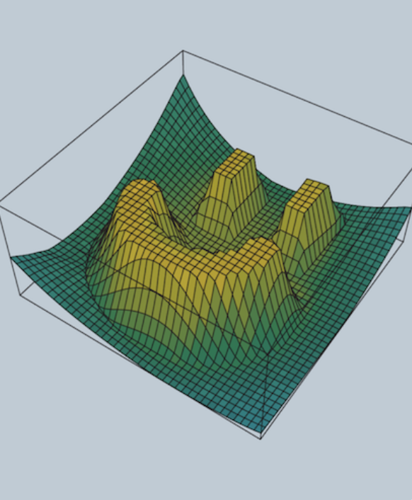
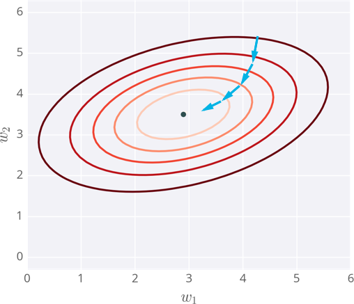
Below I’ve plotted an example of the error of a neural network with two inputs, and accordingly, two weights. You can read this like a topographical map where points on a contour line have the same error and darker contour lines correspond to larger errors.

At each step, you calculate the error and the gradient, then use those to determine how much to change each weight. Repeating this process will eventually find weights that are close to the minimum of the error function, the black dot in the middle.

Caveats

Since the weights will just go wherever the gradient takes them, they can end up where the error is low, but not the lowest. These spots are called local minima. If the weights are initialized with the wrong values, gradient descent could lead the weights into a local minimum, illustrated below.

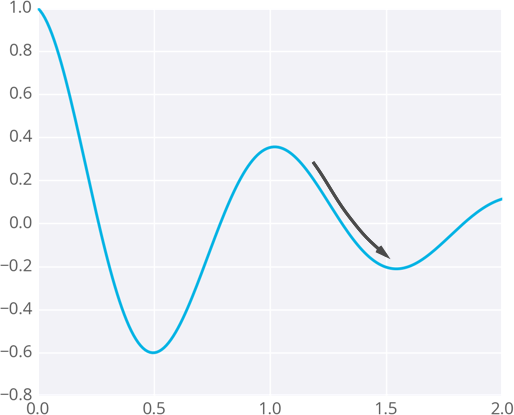
There are methods to avoid this, such as using momentum

Gradient Descent: The Math

Now we know how to get an output from a simple neural network like the one shown here.

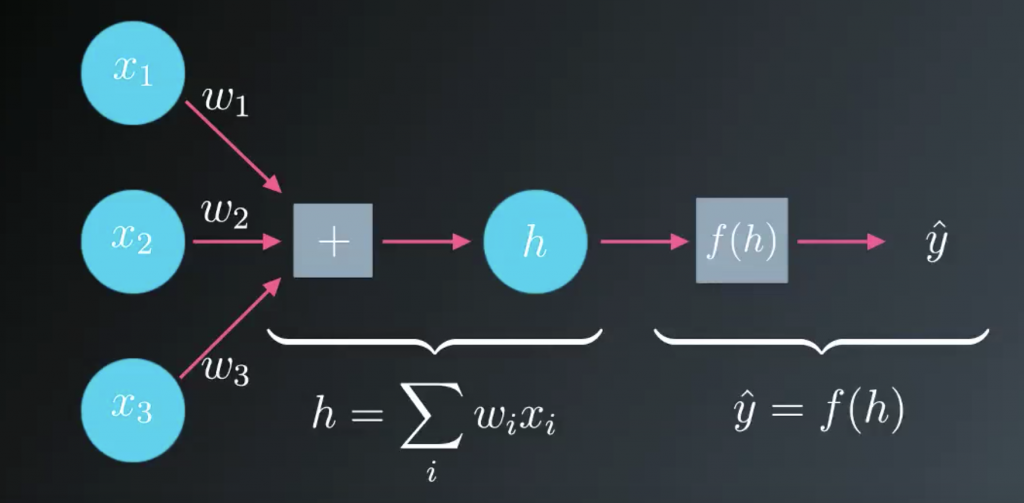
We’d like to use the output to make predictions, but how do we build this network to make predictions without knowing the correct weights before hand? What we can is present it with data that we know to be true then set the model parameters, the weights to match that data. First we need some measure of how bad our predictions are. The obvious choice is to use the difference between the true target value, y, and the network output, y hat.

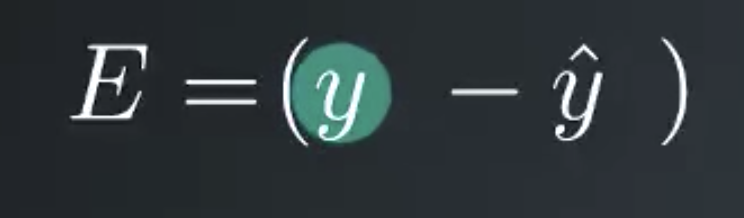
However, if the prediction is too high, this error will be negative and if their prediction is too low by the same amount the error will be positive. We’d rather treat these errors the same to make both cases positive we’ll just square the error. You might be wondering why not just take the absolute value. One bit of using the square is that it penalizes outliers more than small errors.

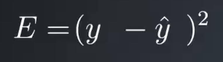
Also squaring the error makes the math nice later. This is the error for just one prediction though. We’d rather like to know the error for the entire dataset. So we’ll just sum up the errors for each data record denoted by the sum over mu. Now we have the total error for the network over the entire dataset. And finally, we’ll add a one half in front because it cleans up the math later.

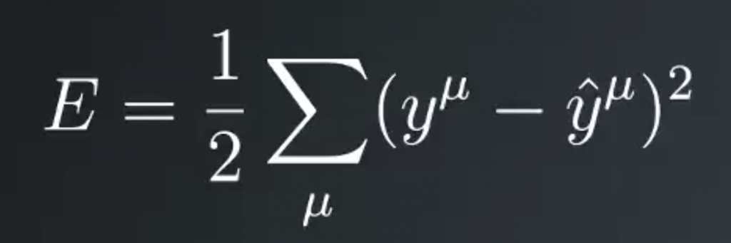
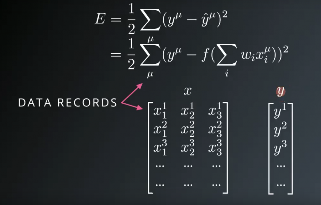
This formulation is typically called the sum of the squared errors (SSE). Remember that y hat is the linear combination of the weights and inputs passed through that activation function. We can substitute it in here, then we see that the error depends on the weights, wi, and the input values, xi.

You can think of the data as two tables or arrays, or matrices, whatever works for you. One contains the input data, x, and the other contains the targets, y. Each record is one row here, so mu equals 1 is the first row. Then, to calculate the total error, you’re just scanning through the rows of these arrays and calculating the SSE. Then summing up all of those results. The SSE is a measure of our network’s performance.

If it’s high, the network is making bad predictions. If it’s low, the network is making good predictions. So we want to make it as small as possible. Going forward, let’s consider a simple example with only one data record to make it easier to understand how we’ll minimize the error. For the simple network the SSE is the true target minus the prediction, y- y hat and squared and divided by 2. Substituting for the prediction, you see the error is a function of the weights. Then our goal is to find weights that minimize the error.

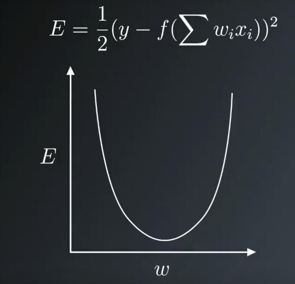
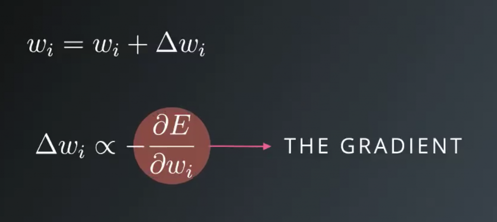
Our goals is to find the weight at the bottom of this bowl. Starting at some random weight, we want to make a step in the direction towards the minimum. This direction is the opposite to the gradient, the slope. If we take many steps, always descending down a gradient. Eventually the weight will find the minimum of the error function and this is gradient descent. We want to update the weight, so a new weight, wi, is the old weight, wi plus this weight step, delta wi. This Greek letter, delta, typically signifies change

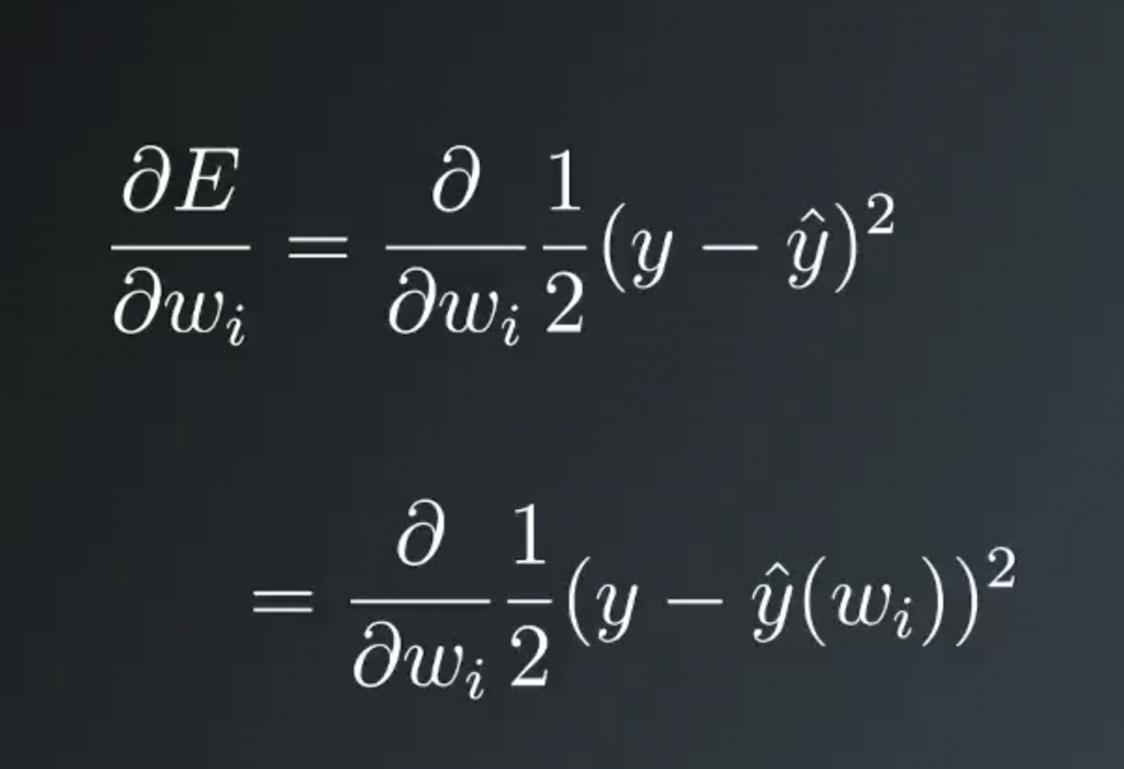
Writing out the gradient, you get the partial derivative with respect to the weights of the squared error. The network output, y hat, is a function of the weights. So what we have here is a function of another function that depends on the weights.

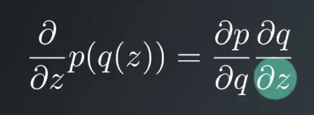
This requires using the chain rule to calculate the derivative. Here is a quick refresher on the chain rule. Say you want to take the derivative of a function p with respect to z. If p depends on another function q that depends on z. The chain rule says, you first take the derivative of p with the respect to q, then multiply it by the derivative of q with the respect to z.

This relates to our problem because we can set q to the error, y- y hat and set p to the squared error. And then we’re taking the derivative with respect to wi, the derivative of p with respect to q returns the error itself. The 2 in the exponent drops down and cancels out the 1/2.

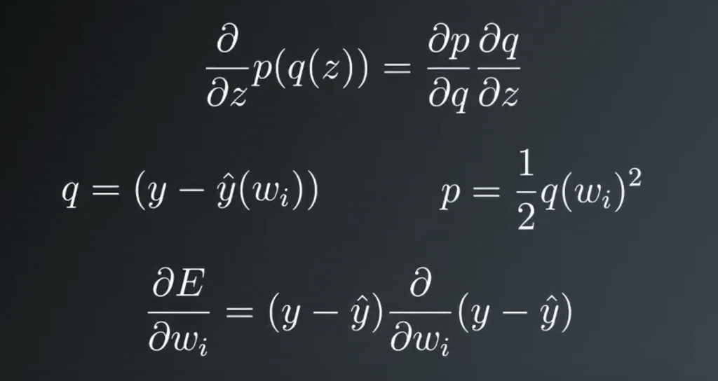
Then we’re left with the derivative of the error with respect to wi. The target value y doesn’t depend on the weights, but y hat does. Using the Chain Rule again, the minus sign comes out in front and we’re left with the partial derivative of y hat. If you remember, y hat is equal to the activation function at h. Where h is the linear combination of the weights and input values.

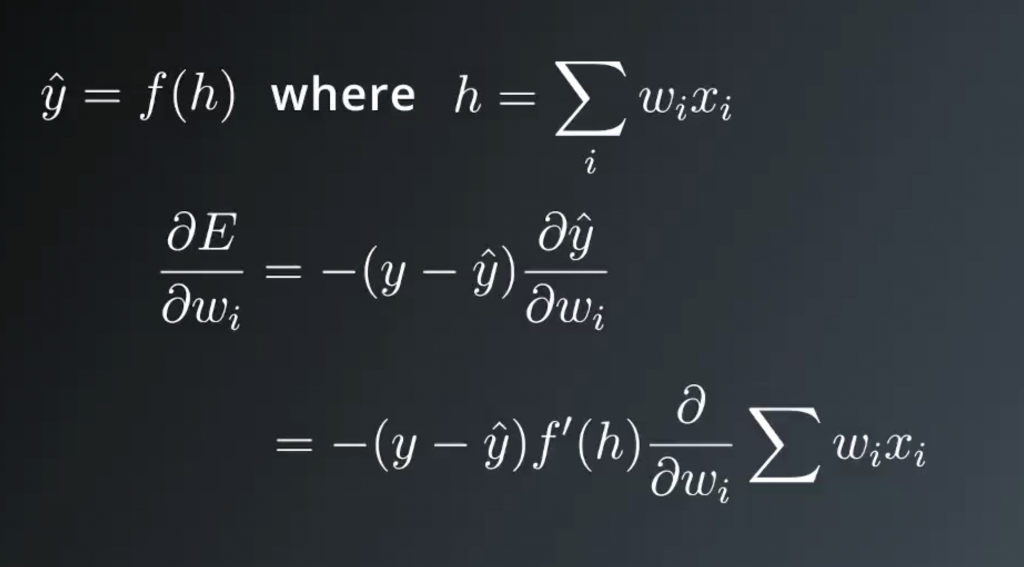
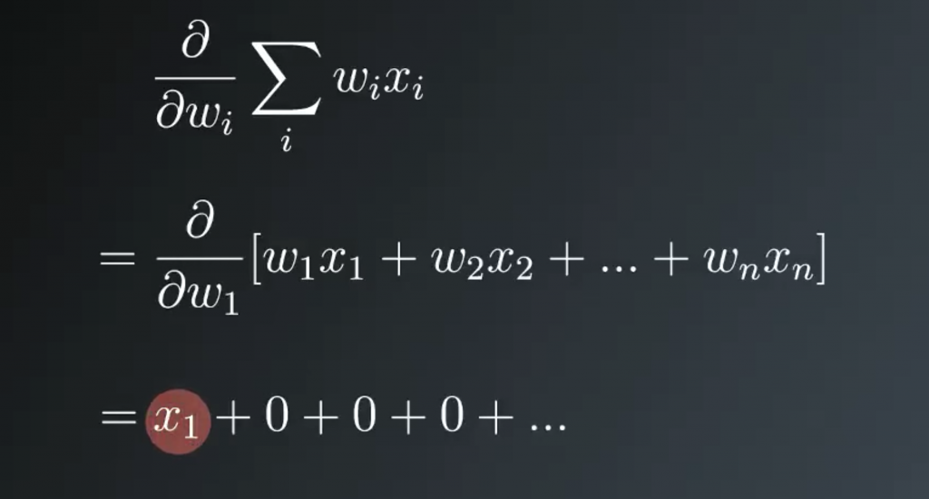
Taking the derivative of y hat, and again using the chain rule. You get the derivative of the activation function at h, times the partial derivative of the linear combination. In the sum, there is only one term that depends on each weight. Writing this out for weight one, you see that only the first term with x1 depends on weight one. Then the partial derivative of the sum with respect to weight one is just x1. All the other terms are zero, then the partial derivative of this sum with respect to wi is just xi.

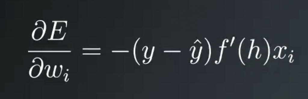
Finally, putting all this together, the gradient of the squared error with respect to wi is the negative of the error times the derivative of the activation function at h times the input value xi.

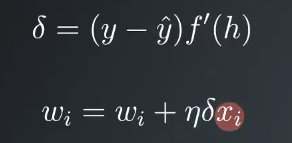
Then the weight step is a learning rate eta times the error, times the activation derivative, times the input value. For convenience, and to make things easy later, we can define an error term, lowercase delta, as the error times the activation function derivative at h. Then we can write our weight update as wi equals wi plus the learning rate times the error term times xi is the value of input i.

You might be working with multiple output units. You can think of this as just stacking the architecture from the single output network but connecting the input units to the new output units. Now the total error would include the error of each outputs sum together. The gradient descent step can be extended to a network with multiple output. By calculating an error term for each output unit denoted with the subscript j

hand-on lab –> http://14.232.166.121:8880/lab? > deeplearning>implement_gradient_descent> gradient_basic.ipynb & gradient.ipynb

Multilayer Perceptrons

Below, we are going to walk through the math of neural networks in a multilayer perceptron. With multiple perceptrons, we are going to move to using vectors and matrices. To brush up, be sure to view the following:

1. Khan Academy’s introduction to vectors.
2. Khan Academy’s introduction to matrices.

Derivation

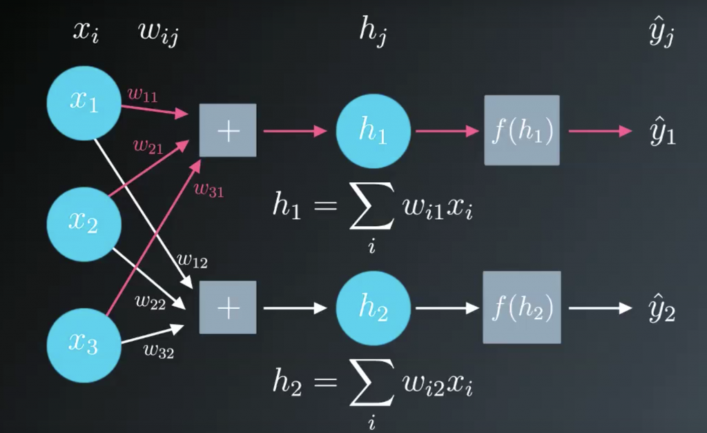
Before, we were dealing with only one output node which made the code straightforward. However now that we have multiple input units and multiple hidden units, the weights between them will require two indices: wij​ where i denotes input units and j are the hidden units.
For example, the following image shows our network, with its input units labeled x1​,x2​, and x3​, and its hidden nodes labeled h1​ and h2​:

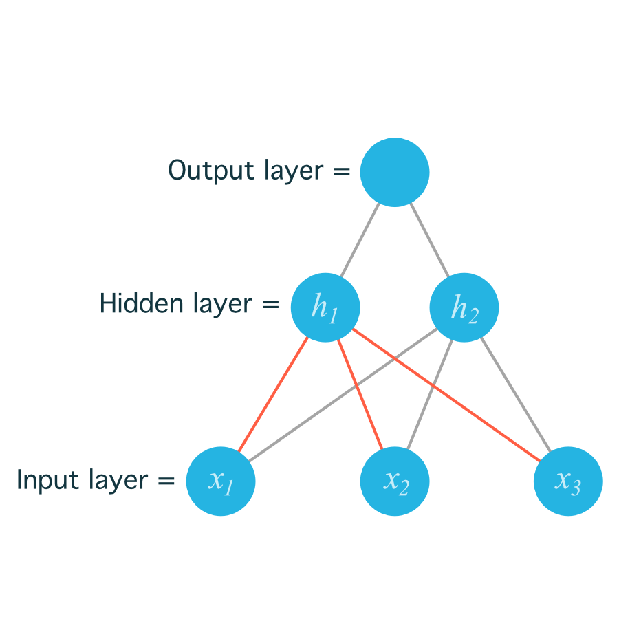
The lines indicating the weights leading to h1​ have been colored differently from those leading to h2​just to make it easier to read.

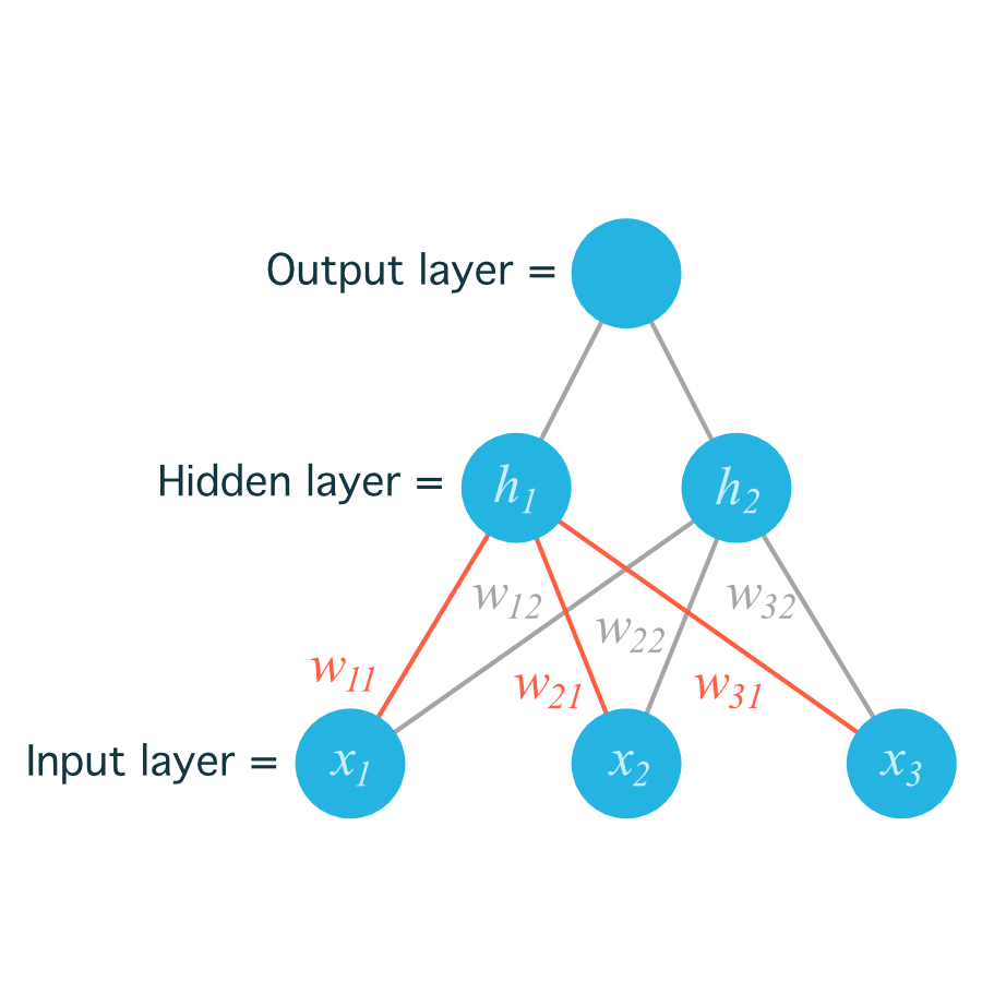
Now to index the weights, we take the input unit number for the i​ and the hidden unit number for the j​. That gives us w11​

for the weight leading from x1​ to h1​, and w12​

for the weight leading from x1​ to h2​.

The following image includes all of the weights between the input layer and the hidden layer, labeled with their appropriate wij​ indices:

Before, we were able to write the weights as an array, indexed as w_iwi​.

But now, the weights need to be stored in a matrix, indexed as w_{ij}wij​. Each row in the matrix will correspond to the weights leading out of a single input unit, and each column will correspond to the weights leading in to a single hidden unit. For our three input units and two hidden units, the weights matrix looks like this:

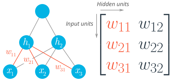
Be sure to compare the matrix above with the diagram shown before it so you can see where the different weights in the network end up in the matrix.

To initialize these weights in NumPy, we have to provide the shape of the matrix. If features is a 2D array containing the input data:

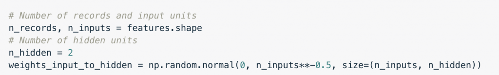
This creates a 2D array (i.e. a matrix) named weights_input_to_hidden with dimensions n_inputsby n_hidden. Remember how the input to a hidden unit is the sum of all the inputs multiplied by the hidden unit’s weights. So for each hidden layer unit, h_jhj​, we need to calculate the following:

To do that, we now need to use matrix multiplication. If your linear algebra is rusty, I suggest taking a look at the suggested resources in the prerequisites section. For this part though, you’ll only need to know how to multiply a matrix with a vector.

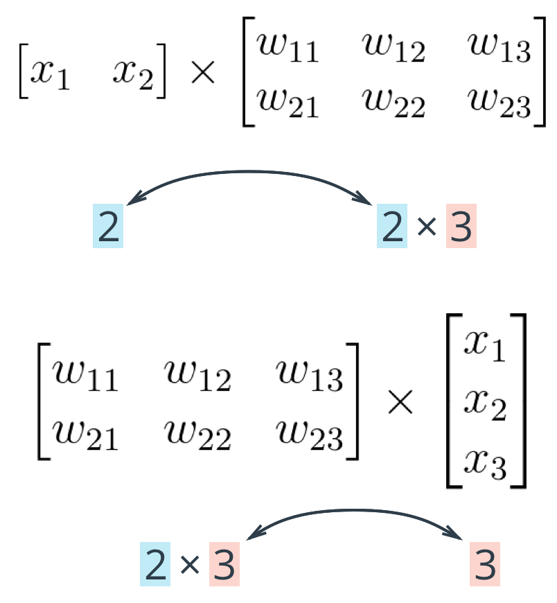
In this case, we’re multiplying the inputs (a row vector here) by the weights. To do this, you take the dot (inner) product of the inputs with each column in the weights matrix. For example, to calculate the input to the first hidden unit, j = 1, you’d take the dot product of the inputs with the first column of the weights matrix, like so:

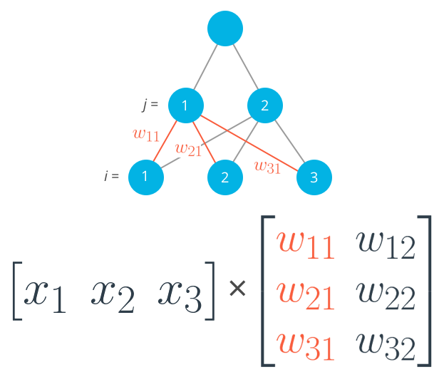
Calculating the input to the first hidden unit with the first column of the weights matrix

And for the second hidden layer input, you calculate the dot product of the inputs with the second column. And so on and so forth.

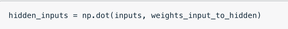
In NumPy, you can do this for all the inputs and all the outputs at once using np.dot

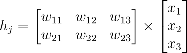
You could also define your weights matrix such that it has dimensions n_hidden by n_inputs then multiply like so where the inputs form a column vector:

Note: The weight indices have changed in the above image and no longer match up with the labels used in the earlier diagrams. That’s because, in matrix notation, the row index always precedes the column index, so it would be misleading to label them the way we did in the neural net diagram. Just keep in mind that this is the same weight matrix as before, but rotated so the first column is now the first row, and the second column is now the second row. If we were to use the labels from the earlier diagram, the weights would fit into the matrix in the following locations:

Remember, the above is not a correct view of the indices, but it uses the labels from the earlier neural net diagrams to show you where each weight ends up in the matrix.

The important thing with matrix multiplication is that the dimensions match. For matrix multiplication to work, there has to be the same number of elements in the dot products. In the first example, there are three columns in the input vector, and three rows in the weights matrix. In the second example, there are three columns in the weights matrix and three rows in the input vector. If the dimensions don’t match, you’ll get this:

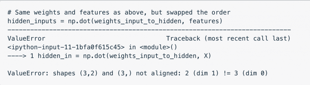
The dot product can’t be computed for a 3×2 matrix and 3-element array. That’s because the 2 columns in the matrix don’t match the number of elements in the array. Some of the dimensions that could work would be the following:

The rule is that if you’re multiplying an array from the left, the array must have the same number of elements as there are rows in the matrix. And if you’re multiplying the matrix from the left, the number of columns in the matrix must equal the number of elements in the array on the right.

Making a column vector

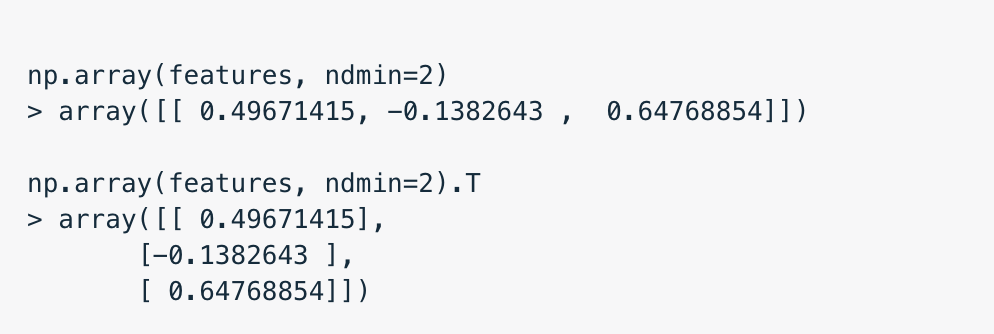
You see above that sometimes you’ll want a column vector, even though by default NumPy arrays work like row vectors. It’s possible to get the transpose of an array like so arr.T, but for a 1D array, the transpose will return a row vector. Instead, use arr[:,None] to create a column vector:

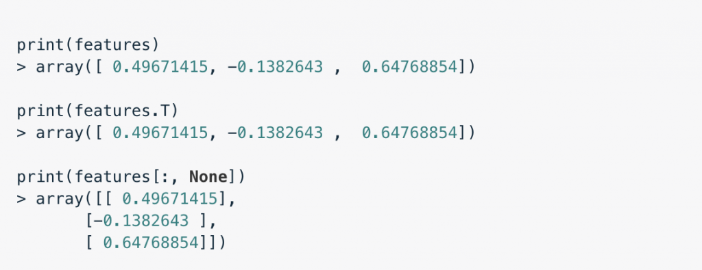
Alternatively, you can create arrays with two dimensions. Then, you can use arr.T to get the column vector.

hand-on lab –> http://14.232.166.121:8880/lab? > deeplearning>implement_gradient_descent> multilayer.ipynb

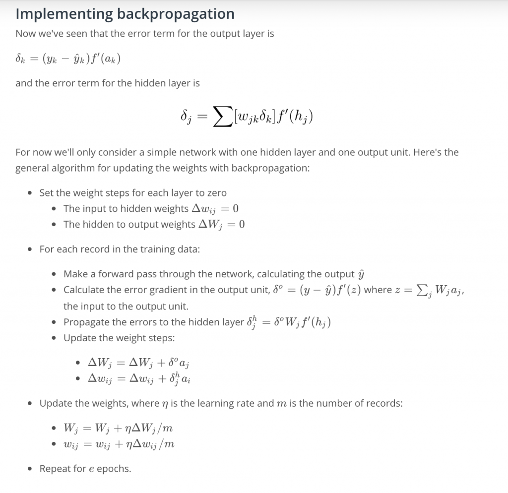
Backpropagation

Now we’ve come to the problem of how to make a multilayer neural network learn. Before, we saw how to update weights with gradient descent. The backpropagation algorithm is just an extension of that, using the chain rule to find the error with the respect to the weights connecting the input layer to the hidden layer (for a two layer network).

To update the weights to hidden layers using gradient descent, you need to know how much error each of the hidden units contributed to the final output. Since the output of a layer is determined by the weights between layers, the error resulting from units is scaled by the weights going forward through the network. Since we know the error at the output, we can use the weights to work backwards to hidden layers.

For example, in the output layer, you have errors δko​ attributed to each output unit k. Then, the error attributed to hidden unit j is the output errors, scaled by the weights between the output and hidden layers (and the gradient):

Then, the gradient descent step is the same as before, just with the new errors:

where wij​ are the weights between the inputs and hidden layer and xi​ are input unit values. This form holds for however many layers there are. The weight steps are equal to the step size times the output error of the layer times the values of the inputs to that layer

Here, you get the output error, δoutput​, by propagating the errors backwards from higher layers. And the input values, Vin​ are the inputs to the layer, the hidden layer activations to the output unit for example.

Working through an example

Let’s walk through the steps of calculating the weight updates for a simple two layer network. Suppose there are two input values, one hidden unit, and one output unit, with sigmoid activations on the hidden and output units. The following image depicts this network. (Note: the input values are shown as nodes at the bottom of the image, while the network’s output value is shown as y^​ at the top. The inputs themselves do not count as a layer, which is why this is considered a two layer network.)

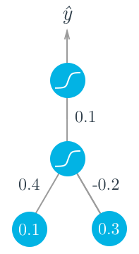
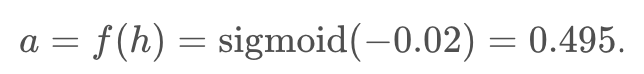
Assume we’re trying to fit some binary data and the target is y = 1y=1. We’ll start with the forward pass, first calculating the input to the hidden unit

and the output of the hidden unit

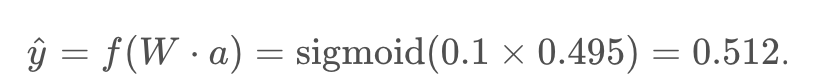
Using this as the input to the output unit, the output of the network is

With the network output, we can start the backwards pass to calculate the weight updates for both layers.  the error term for the output unit is

Now that we have the errors, we can calculate the gradient descent steps. The hidden to output weight step is the learning rate, times the output unit error, times the hidden unit activation value.

Then, for the input to hidden weights w_iwi​, it’s the learning rate times the hidden unit error, times the input values.

From this example, you can see one of the effects of using the sigmoid function for the activations. The maximum derivative of the sigmoid function is 0.25, so the errors in the output layer get reduced by at least 75%, and errors in the hidden layer are scaled down by at least 93.75%! You can see that if you have a lot of layers, using a sigmoid activation function will quickly reduce the weight steps to tiny values in layers near the input. This is known as the vanishing gradient problem. Later in the course you’ll learn about other activation functions that perform better in this regard and are more commonly used in modern network architectures.

hand-on lab –> http://14.232.166.121:8880/lab? > deeplearning>implement_gradient_descent> backprop_basic.ipynb & backprop.ipynb

Further reading

Backpropagation is fundamental to deep learning. TensorFlow and other libraries will perform the backprop for you, but you should really really understand the algorithm. We’ll be going over backprop again, but here are some extra resources for you:

• From Andrej Karpathy: Yes, you should understand backprop
• Also from Andrej Karpathy, a lecture from Stanford’s CS231n course