Introduction

A hyper parameter is a variable that we need to set before applying a learning algorithm into a dataset. The challenge with hyper parameters is that there are no magic numbers that work everywhere. The best numbers depend on each task and each dataset. Generally speaking, we can break hyper parameters down into two categories. The first category is optimizer hyper parameters.

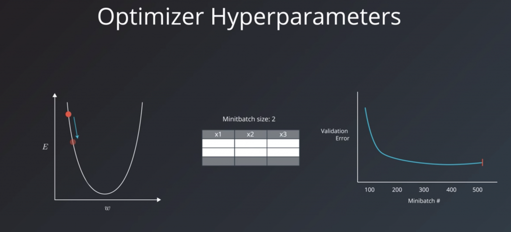
These are the variables related more to the optimization and training process than to the model itself. These include the learning rate, the minibatch size, and the number of training iterations or epochs.

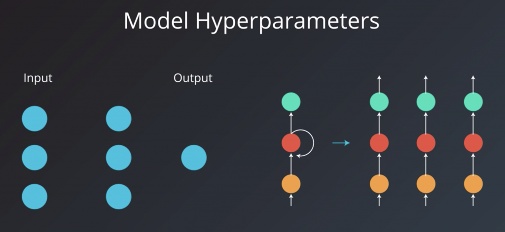
The second category is model hyper parameters. These are the variables that are more involved in the structure of the model. These include the number of layers and hidden units and model specific hyper parameters for architectures like RNMs.

Learning Rate

The learning rate is the most important hyperparameter. Even if you apply models that other people built to your own dataset, you’ll find that you’ll probably have to try a number of different values for the learning rate to get the model to train properly. If you took care to normalize the inputs to your model, then a good starting point is usually 0.01. And these are the usual suspects of learning rates. If you try one and your model doesn’t train, you can try the others. Which of the others should you try? That depends on the behavior of the training error. To better understand this, we’ll need to look at the intuition of the learning rate. we saw that when we use gradient descent to train a neural network model, the training task boils down to decreasing the error value calculated by a loss function as much as we can. During a learning step, we do a calculate the loss, then find the gradient.

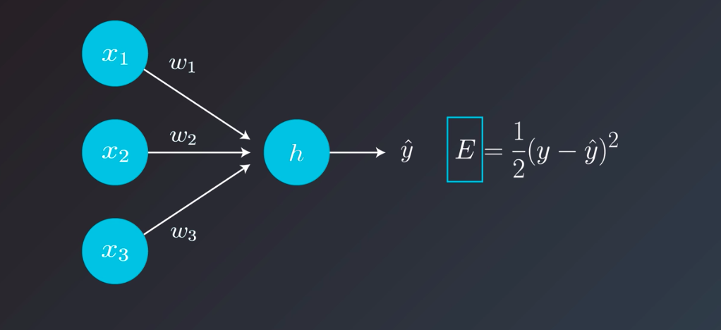
Let’s assume this simplest case, in which our model has only one weight. The gradient will tell us which way to nudge the current weight so that our predictions become more accurate. To visualize the dynamics of the learning rate; let take a look at some situations depicted in the following:

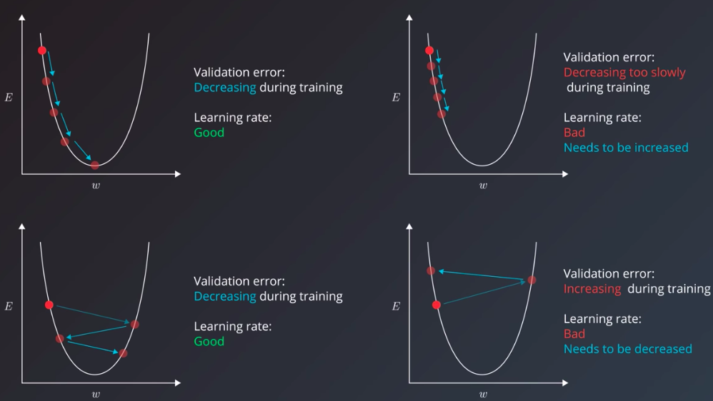
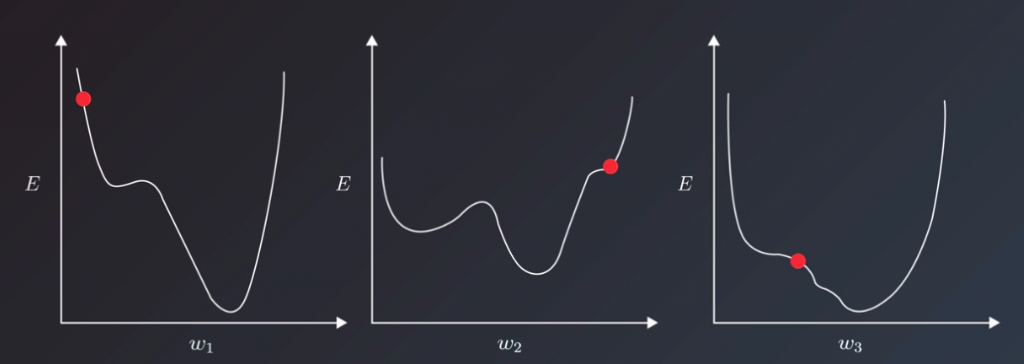
this here is a simple example with only one parameter, and an ideal convex error curve. Things are more complicated in the real world, I’m sure you’ve seen your models are likely to have hundreds or thousands of parameters, each with its own error curve that changes as the values of the other weights change. And the learning rate has to shepherd all of them to the best values that produce the least error. To make matters even more difficult for us, we don’t actually have any guarantees that the error curves would be clean u-shapes. They might, in fact, be more complex shapes with local minima that the learning algorithm can mistake for the best values and converge on.

Now that we looked at the intuition of the learning rates, and the indications that the training error gives us that can help us tune the learning rate, let’s look at one specific case we can often face when tuning the learning rate. Think of the case where we chose a reasonable learning rate. It manages to decrease the error, but up to a point, after which it’s unable to descend, even though it didn’t reach the bottom yet. It would be stuck oscillating between values that still have a better error value than when we started training, but are not the best values possible for the model. This scenario is where it’s useful to have our training algorithm decrease the learning rate throughout the training process. This is a technique called learning rate decay. Some adaptive learning optimizers are AdamOptimizer or AdagradOptimizer

Minibatch Size

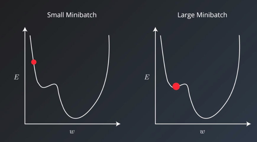
Minibatch size is another hyper parameter that no doubt you’ve run into a number of times already. It has an effect on the resource requirements of the training process but also impacts training speed and number of iterations in a way that might not be as trivial as you may think. It’s important to review a little bit of terminology here first. Historically there had been debate on whether it’s better to do online also called stochastic training where you fit a single example of the dataset to the model during a training step. And using only one example, do a forward pass, calculate the error, and then back propagate and set adjusted values for all your parameters. And then do this again for each example in the dataset. Or if it was better to feed the entire dataset to the training step and calculate that gradient using the error generated by looking at all the examples in the dataset. This is called batch training. The abstraction commonly used today is to set a minibatch size. So online training is when the minibatch size is one, and batch training is when the minibatch size is the same as the number of examples in the training set. And we can set the minibatch size to any value between these two values. The recommended starting values for your experimentation are between one and a few hundred with 32 often being a good candidate. A larger minibatch size allows computational boosts that utilizes matrix multiplication, in the training calculations. But that comes at the expense of needing more memory. In practice, small minibatch sizes have more noise in their error calculations, and this noise is often helpful in preventing the training process from stopping at local minima on the error curve rather than the global minima that creates the best model.

This is an experimental result for the effective batch size on convolutional neural nets

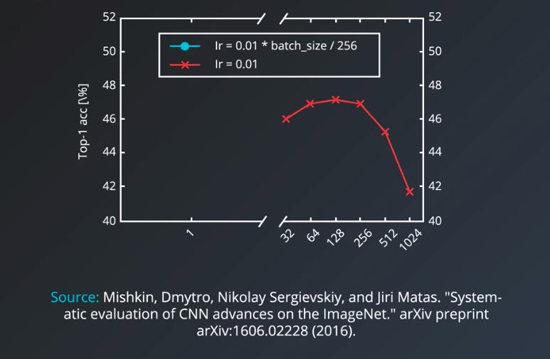
It shows that using the same learning rate, the accuracy of the model decreases the larger the minibatch size becomes.

Number of Training Iterations / Epochs

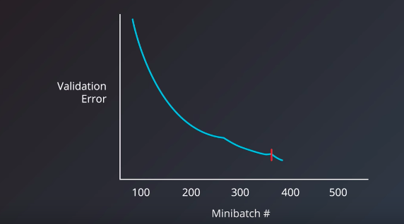
To choose the right number of iterations or number of epochs for our training step, the metric we should have our eyes on is the validation error. The intuitive manual way is to have the model train for as many epochs or iterations that it takes, as long as the validation error keeps decreasing. Luckily, however, we can use a technique called early stopping to determine when to stop training a model. Early stopping roughly works by monitoring the validation error, and stopping the training when it stops decreasing.

Number of Hidden Units / Layers

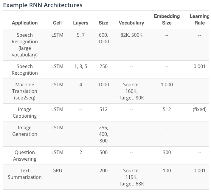
Let’s now talk about the hyperparameters that relates to the model itself rather than the training or optimization process. The number of hidden units, in particular, is the hyperparameter I felt was the most mysterious when I started learning about machine learning. The main requirement here is to set a number of hidden units that is “large enough”. For a neural network to learn to approximate a function or a prediction task, it needs to have enough “capacity” to learn the function. The more complex the function, the more learning capacity the model will need. The number and architecture of the hidden units is the main measure for a model’s learning capacity. If we provide the model with too much capacity, however, it might tend to overfit and just try to memorize the training set. If you find your model overfitting your data, meaning that the training accuracy is much better than the validation accuracy, you might want to try to decrease the number of hidden units. You could also utilize regularization techniques like dropouts or L2 regularization. So, as far as the number of hidden units is concerned, the more, the better. A little larger than the ideal number is not a problem, but a much larger value can often lead to the model overfitting. So, if your model is not training, add more hidden units and track validation error. Keep adding hidden units until the validation starts getting worse. Another heuristic involving the first hidden layer is that setting it to a number larger than the number of the inputs has been observed to be beneficial in a number of tests. What about the number of layers? Andrej Karpathy tells us that in practice, it’s often the case that a three-layer neural net will outperform a two-layer net, but going even deeper rarely helps much more. The exception to this is convolutional neural networks where the deeper they are, the better they perform.

LSTM Vs GRU

“These results clearly indicate the advantages of the gating units over the more traditional recurrent units. Convergence is often faster, and the final solutions tend to be better. However, our results are not conclusive in comparing the LSTM and the GRU, which suggests that the choice of the type of gated recurrent unit may depend heavily on the dataset and corresponding task.”

Empirical Evaluation of Gated Recurrent Neural Networks on Sequence Modeling by Junyoung Chung, Caglar Gulcehre, KyungHyun Cho, Yoshua Bengio

“The GRU outperformed the LSTM on all tasks with the exception of language modelling”

An Empirical Exploration of Recurrent Network Architectures by Rafal Jozefowicz, Wojciech Zaremba, Ilya Sutskever

“Our consistent finding is that depth of at least two is beneficial. However, between two and three layers our results are mixed. Additionally, the results are mixed between the LSTM and the GRU, but both significantly outperform the RNN.”

Visualizing and Understanding Recurrent Networks by Andrej Karpathy, Justin Johnson, Li Fei-Fei

“Which of these variants is best? Do the differences matter? Greff, et al. (2015) do a nice comparison of popular variants, finding that they’re all about the same. Jozefowicz, et al. (2015) tested more than ten thousand RNN architectures, finding some that worked better than LSTMs on certain tasks.”

Understanding LSTM Networks by Chris Olah

“In our [Neural Machine Translation] experiments, LSTM cells consistently outperformed GRU cells. Since the computational bottleneck in our architecture is the softmax operation we did not observe large difference in training speed between LSTM and GRU cells. Somewhat to our surprise, we found that the vanilla decoder is unable to learn nearly as well as the gated variant.”

Massive Exploration of Neural Machine Translation Architectures by Denny Britz, Anna Goldie, Minh-Thang Luong, Quoc Le

Resource and Reference

If you want to learn more about hyperparameters, these are some great resources on the topic:

• Practical recommendations for gradient-based training of deep architectures by Yoshua Bengio
• Deep Learning book – chapter 11.4: Selecting Hyperparameters by Ian Goodfellow, Yoshua Bengio, Aaron Courville
• Neural Networks and Deep Learning book – Chapter 3: How to choose a neural network’s hyper-parameters? by Michael Nielsen
• Efficient BackProp (pdf) by Yann LeCun

More specialized sources:

• How to Generate a Good Word Embedding? by Siwei Lai, Kang Liu, Liheng Xu, Jun Zhao
• Systematic evaluation of CNN advances on the ImageNet by Dmytro Mishkin, Nikolay Sergievskiy, Jiri Matas
• Visualizing and Understanding Recurrent Networks by Andrej Karpathy, Justin Johnson, Li Fei-Fei