Part of speech Tagging with HMMs
Part of Speech Tagging
Okay, here’s the problem we’re going to solve in this section We have a sentence, for example, “Mary had a little lamb”, and we need to figure out which words are nouns, verbs, adjectives, adverbs, et cetera. Now, a thorough knowledge in grammar is not needed in this section only to know that words are normally given these labels or tags. For this sentence, the tags are noun for Mary, verb for had, determinant for a, adjective for little, and again noun for lamb. These labels are called parts of speech and so this problem is called part-of-speech tagging,
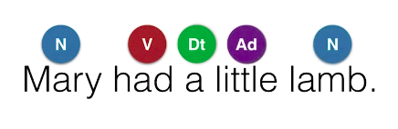
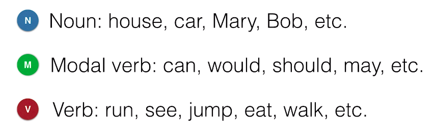
and what we’ll do in this post is develop some models that will help us label these words with their corresponding part of speech based on existing label data. The main model that we’ll learn today is a hidden Markov model. So for simplicity, in this section we’ll only be using three parts of speech. Along in the project, you’ll use more. The ones we’ll use are noun. So, things like house, car, Mary, Bob, et cetera. Then, we have a modal verb, which is normally used with another verb. These are words like can, would, should, may, et cetera. And finally, we’ll have verbs, which are actions like run, see, jump, eat, walk, et cetera.
Lookup Table
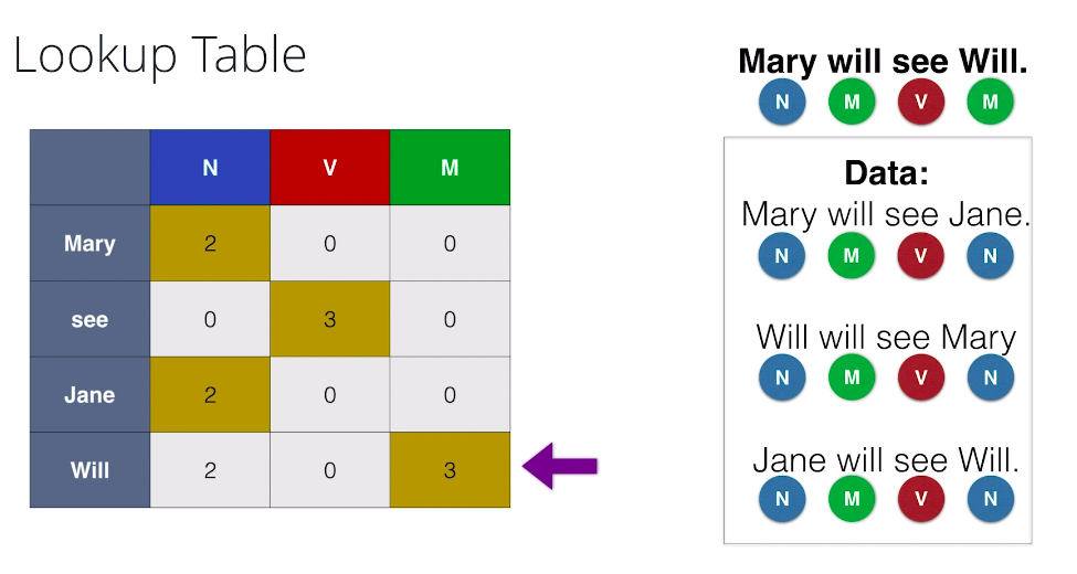
So, let’s start with some friends. Let’s say we have our friend, Mary, our friend, Jane, and our friend, Will. And we want to tag the sentence: Mary saw Will. And to figure this out, we have some exciting data in the form of some sentences, which are “Mary saw Jane.”, and “Jane so Will.” And these are tagged as follows.
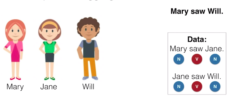
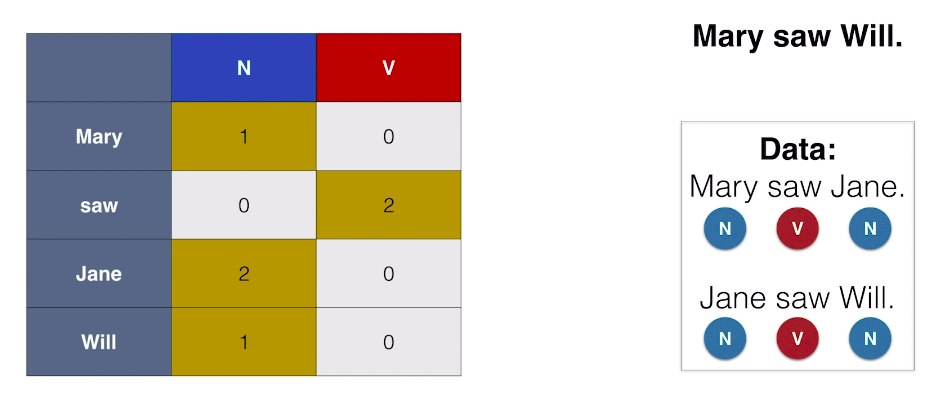
Mary, Jane, and Will are tagged as nouns, and saw is tagged as a verb. On our first algorithm it’s going to be very simple. We’re just going to tag each word with the most common part of speech. So, we make a little table where the rows are the words and the columns are the parts of speech, and we write down how often each one appears in the existing data. the table looks like:
Bigrams
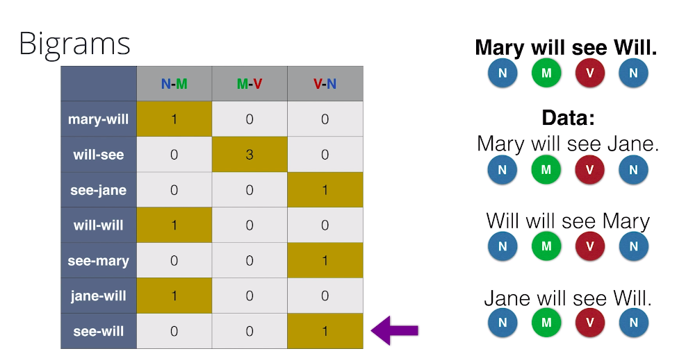
Now, of course we can’t really expect the Lookup Table method to work all the time. Here’s a new example where the sentences are getting a bit more complicated. Now, our data is formed by the sentences, Mary will see Jane, Will will see Mary, and Jane will see Will. And the tags are as follows. Noun, modal, and verb. And our goal is to tag the sentence, Mary will see Will. So we do a normal Lookup Table like this, and let’s tag our sentence. Mary gets correctly tagged as a noun. Then Will, get correctly tagged as a modal.See gets correctly tagged as a verb, and here’s a problem. Will, always get tagged as a modal since it appears three times as modal and two times as a noun, but in this sentence, we know Will is a noun since it’s referring to our friend Will. This is a problem. In particular, Lookup Tables won’t work very well if a word can have two different tags, since it will always pick the most common tags that’s associated with no matter the context.
So now the question is, how do we take the context into account? Well, the simplest way to think of context is to look at each words neighbor. So for instance, if we tag pairs of words. For example, here we tagged the consecutive pair, see-Jane as a verb-noun one time, as it appears once as verb-noun. And now, onto tag other sentence. We’ll tag the first word using the previous table. So let’s tag Mary as a noun. Now, for each following word, we’ll tag using the previous one, and the Lookup Table to find the pair of tags that correspond to them. So for example, to tag the word will, we look at Mary-will in particular where Mary is a noun and we see that the most common one is when will is a modal. So we’ll tag will as a modal. We continue tagging see as a verb, and the second Will correctly as a noun, since the pair see-Will is tagged as a verb-noun.
When bigrams won’t work
Okay. So now let’s complicate the problem a little bit. We still have Mary, Jane and Will. And let’s say there’s a new member of the gang called Spot. And now our data is formed by the following four sentences,
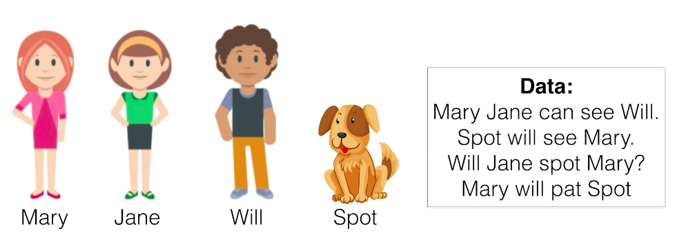
Mary, Jane can see Will. Spot will see Mary. Will Jane spot Mary? And Mary will pat Spot. And we want to tag the sentence, Jane will spot Will. So let’s try a lookup table and I won’t fill it in, but let’s say we can fill it in based on the data. What’s a potential problem here? Well, when we look at the first pair Jane will, we notice that that’s not in the data. This pair of words never appears. But somehow, it’s a pair that makes sense.
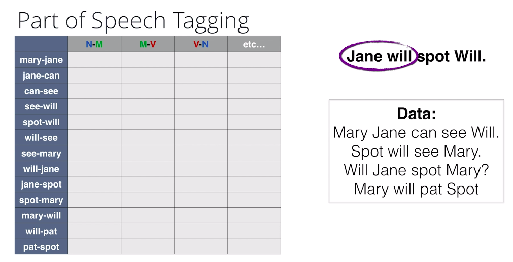
So, a problem with bigrams or n-grams in general is that sometimes every pair or every n-gram doesn’t appear, and then we have no way to fill in the extra information. So for this, we’ll introduce hidden mark of models.
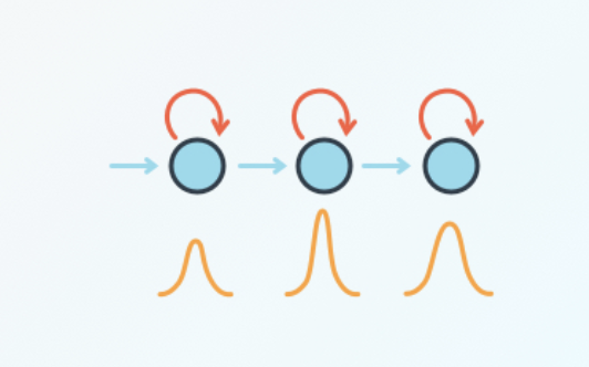
Hidden Markov Models
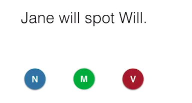
The idea for Hidden Markov Models is the following: Let’s say that a way of tagging the sentence “Jane will spot Will” is noun-modal-verb-noun and we’ll calculate a probability associated with this tagging. So we need two things. First of all, how likely is it that a noun is followed by a modal and a modal by a verb and a verb by a noun. These need to be high in order for this tagging to be likely. These are called the transition probabilities.
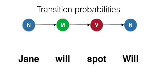
Now, the second set of probabilities we need to calculate are these: What is the probability that a noun will be the word Jane and that a modal will be the word will, etc. This also need to be relatively high for our tagging to be likely. These are called the Emission Probabilities.
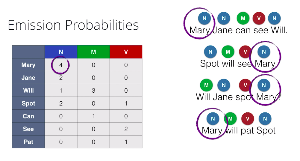
So, here are sentences with their corresponding tags and we’re going to calculate the Emission Probabilities, that is the probability that if a word is, say, a noun that that word will be Mary or Jane, etc. So, to do this we again do a counting table like this one where, for example, the entry on the Mary row and the noun column is four because Mary appears four times as a noun. Now, in order to find the probabilities, we divide each column by the sum of the entries and we obtain the following numbers.
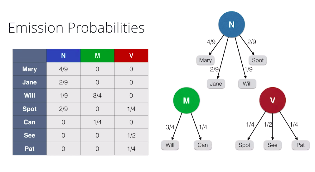
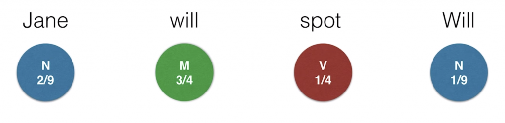
And we also have graphical representation of this table. Say, if we know that a word is a noun, the probabilities of it being Mary is four over nine, Jane is two over nine, Will is one over nine, and Spot is two over nine. The other words are zero. Same thing for modal, and for verb.
So, now let’s calculate the transition probabilities. These are the probabilities that are part of speech follows another part of speech. First, in order to actually get the whole picture, we’ll add starting and ending tags on each sentence and we’ll treat these tags as parts of speech as well. And now we make a table of counts in this table. We count the number of appearances of each pair of parts of speech. For example, this three here in the noun row and the modal column corresponds to the three occurrences of a noun followed by a modal. Now, to find the probabilities, we divide each row by the sum of the entries in the row. And here’s a nice graph of our transition probabilities.
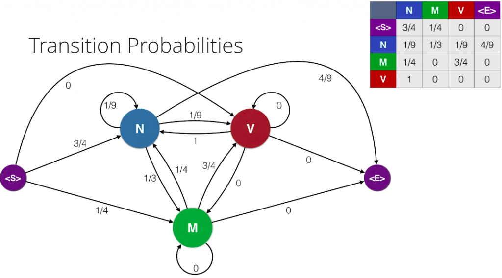
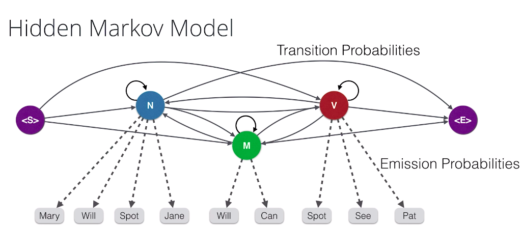
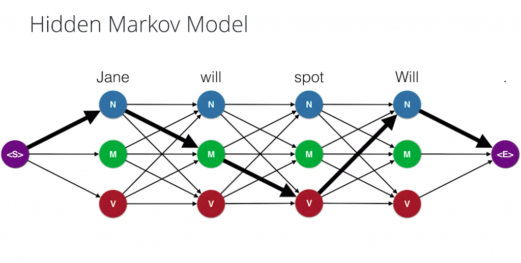
We draw our parts of speech and arrows between them with the transition probabilities attached to them, and as a final step we combine the two previous graphs to form a Hidden Markov Model. We have our words, which are observations. These are called the observations because they are the things we observe when we read the sentences And the parts of speech are called the Hidden States, since they are the ones we don’t know and we have to infer based on the words. And among the Hidden States we have the transmission probabilities, and between the Hidden States and the observation we have the Emission Probabilities. And that’s it. That’s a Hidden Markov Model.
How many paths?
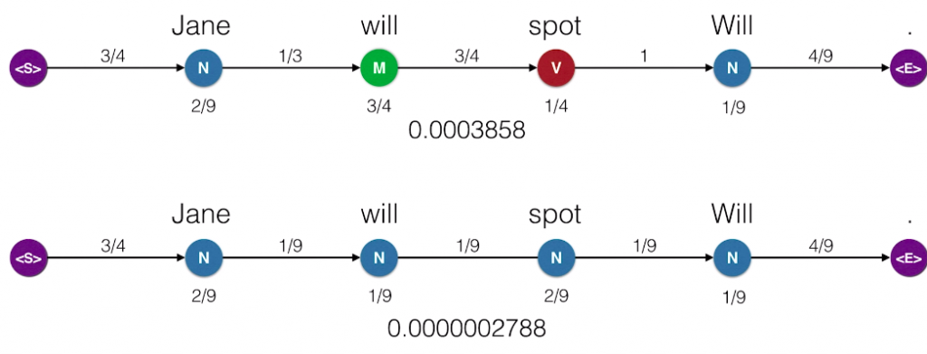
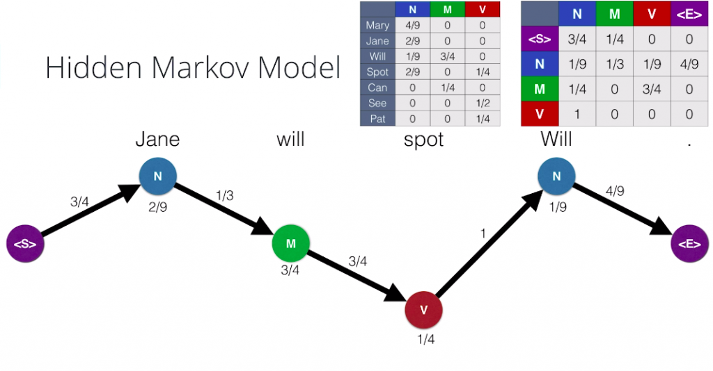
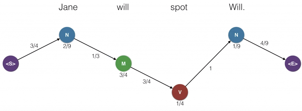
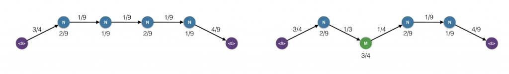
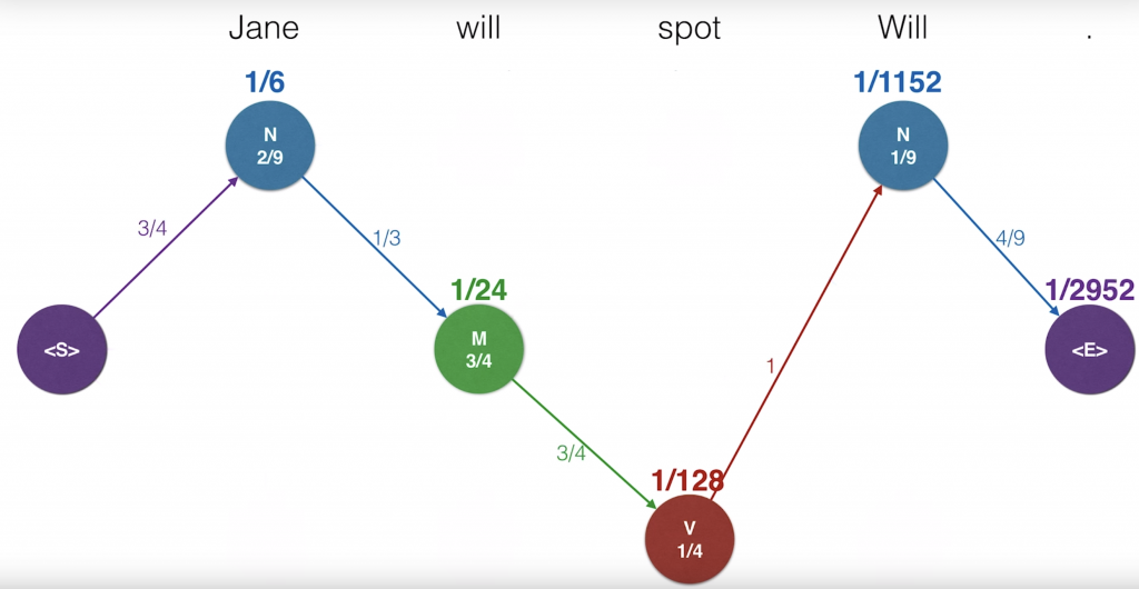
So now, what we’ll do is we’ll record the probability of the sentence being generated. So, we start again at the starting state. And as we remember, we walked to the N. The transition probability from the start state to N is three-quarters. So we’ll record this three-quarters. Now, at N we generate the word Jane. This happens with emission probability two-ninths, so we record that. Now, we move to M and the transition probability is one-third and generate Will with emission probability of three-quarters. Then, we move to V with transition probability three-quarters and generate spot with the emission probability one-quarter. Then, we move back to N with transition probability one and we generate Will with emission probability one over nine. Finally, we move to the end state with transition probability four over nine. So, since the transition moves are all independent of each other and the emission moves are conditional on the hidden state that were located at, the probability that this Hidden Markov Model generates a sentence is the product of these probabilities. We multiply them and get the total probability of the sentence being emitted is 0.0003858. It looks small, but actually it’s large considering the huge amount of sentences we can generate of many lengths. So let’s repeat this path for, Jane will spot Will. We have the parts of speech noun, modal, verb, noun and the probabilities, and their product is 0.0003858. Let’s see if another path can generate this sentence. What about the path noun noun noun noun? We hope this is smaller since it’s a bit of a nonsensical pattern of parts of speech. And indeed, it is very small. It is the product of these numbers which is 0.0000002788. So, among these two, we pick the one on top because it generates the sentence with a higher probability. And in general, what we’ll do is from all the possible combinations of parts of speech, we’ll pick the one that generates the sentence, Jane will spot Will, with the highest probability. This is called maximum likelihood. It’s the core of many algorithms and artificial intelligence. So that’s simple. All we have to do is go over all the possible chains of parts of speech that could generate the sentence.
So, let’s have a small quiz. How many of these chains are there?
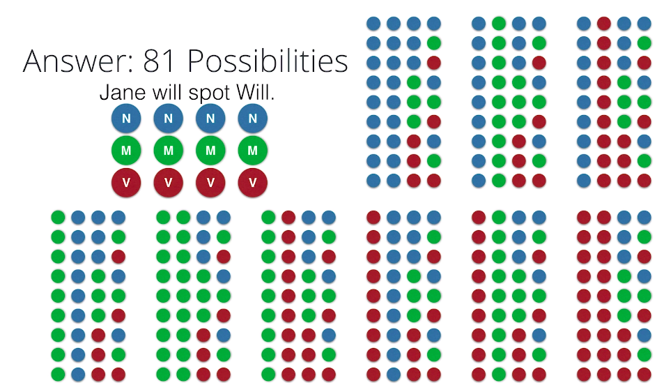
The answer is 81. And the reason is that we have three possibilities forJane, three for will, three for spot, and three for Will. Here are the 81 possibilities. So this is not so bad. We could check 81 products of four things and find the largest one. But what if we have say 30 parts of speech and we need to take a sentence of 10 words. Then we have 30 to the 10 possibilities. That starts being pretty large. In general, it’s exponential and we don’t want to have to check exponentially many things. So, here’s another way to see this 81 combinations as paths.
Here we have our sentence, and here we have our states. The start state and then three choices for each word and then the end state. This gives us the three times three times three times three, which is 81.
Notice that each combination of four states also gives us a path from left to right. For example, the combination noun, modal, verb, noun, gives us this path over here.
Unless we called that for each element in the path vertices and edges, we have a corresponding probability which comes from the emission and the transition probability tables. And then, we multiply these probabilities to get the total probability of the path. So, at the end of the day, what we have to do is find the path from left to right, that gives us the highest probability.
Which path is more likely?
And here are the four paths we have to check
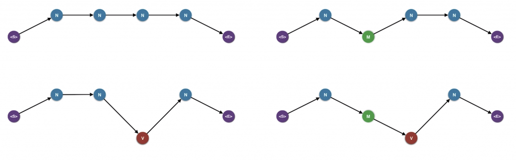
So new quiz. Which one of these gives us the sentence with the highest probability?
Correct. The answer is noun-modal-verb-noun.
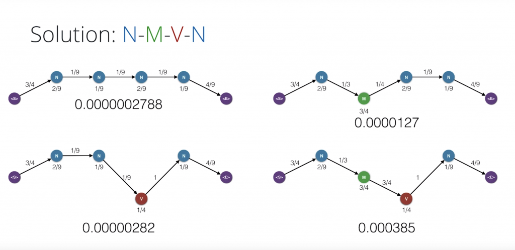
Precisely this one, this is the winner
Viterbi Algorithm Idea
Let’s look at only these two paths and let’s merge them
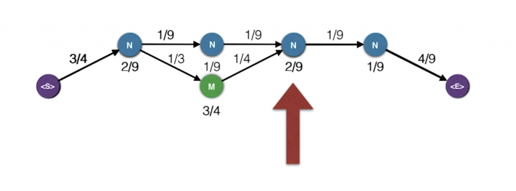
So now, what happens at say this point. There are two ways to get to that point. And here are the two ways. And the probabilities for the mini path in the left is much smaller than that of the mini path on the right. So, we’re really just concerned with the mini path on the right, and we can forget about the other one. At the end of the day, that’s what we want. For every possible state, we will record the highest probability path that ends in that state. This known as the Viterbi algorithm.
Viterbi Algorithm
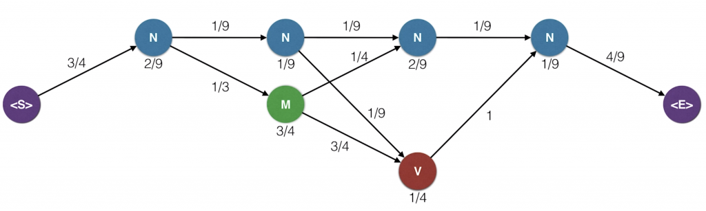
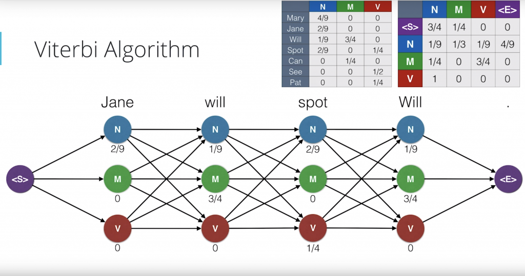
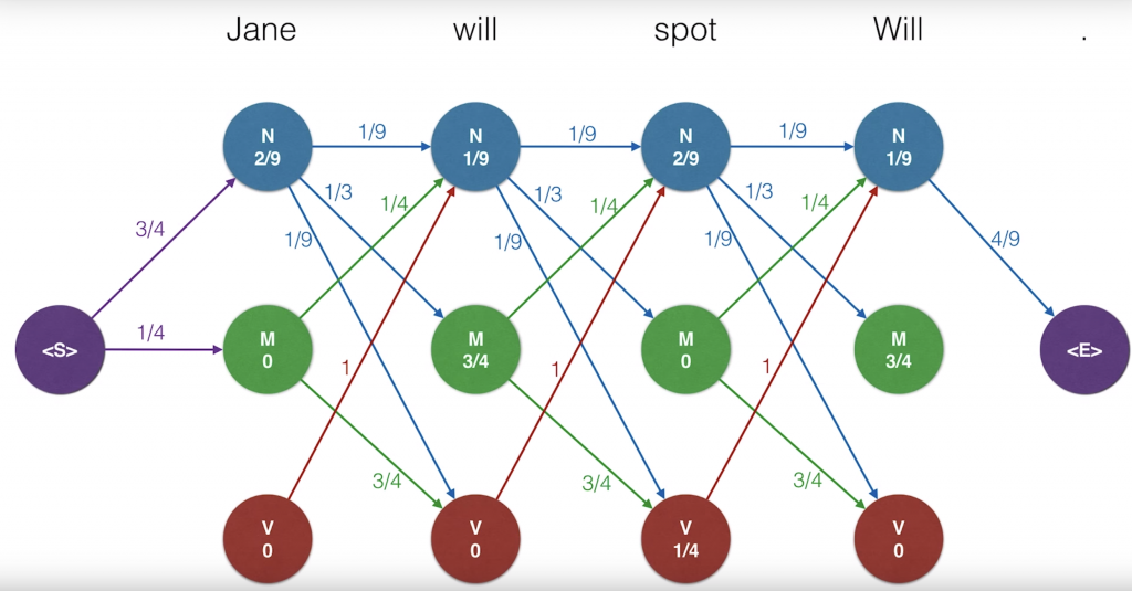
if you’ve seen dynamic programming, that’s exactly what we’re doing. So here’s our trellised diagram with the two probability tables, mission and transition. Let’s draw this a bit larger with all the probabilities. Recall that on each node we have the emission probabilities, so that’s the probability that the particular part of speech generated the word above. And on the edges, we have the transition probabilities which are the probability that we get from one state to the next one. For clarity, we’ve removed the edges that have probability zero but we still consider them. Now, the idea is that for each state or dot in the diagram, Now, the idea is that for each state or dot in the diagram, we will record the maximum probability of all the paths that end in that dot and generate the words that are above.
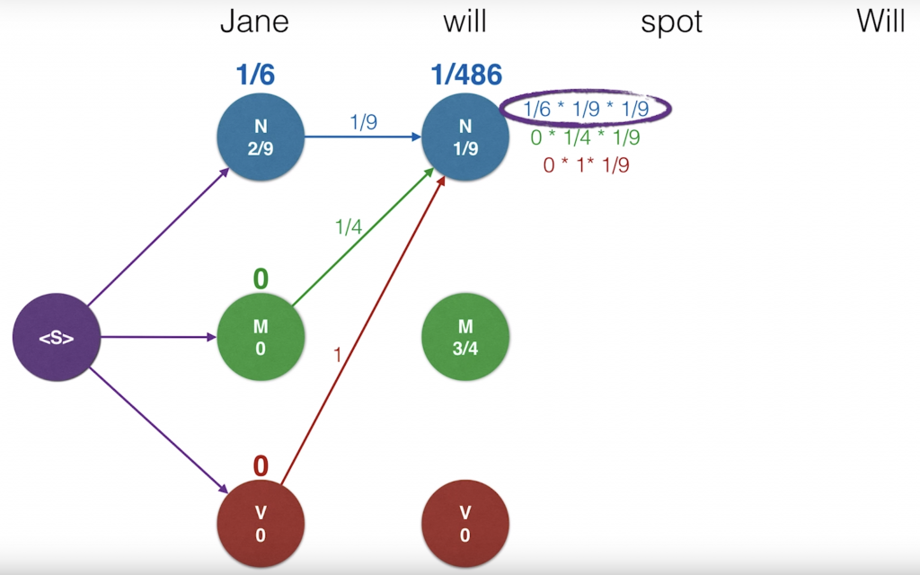
So let’s start from the left. The probability that the word Jane is generated by the path that ends at the top end node is the product of the probability of getting to that node from the start node, which is three quarters, times the probability that the node generated the word Jane which is two over nine. This product is one sixth that was recorded. Likewise, the probability of the M node is one-quarter times zero which is zero and the one on the V node is zero times zero which is zero. Now, let’s go to the next word will. There are three paths that end in the top right N node. One coming from the previous N, one from the previous M and one from the previousV. We need to look at the three and pick the one with the largest probability. The probability for the path coming from the N node is one-sixth, which is a probability so far until the word Jane, times the transition probability one over nine to get to the new N node, times the emission probably one over nine for a emitting the word will. We’ll record this product as one-sixth times one-ninth times one-ninth. Likewise, for the path that comes from the M, the probability is zero times one-quarter times one-ninth And for the path that comes from the V, it’s zero times one times one-ninth. Since two of these are zero, the largest one is the first one which is one over 486.
So we will record that number as the probability of the highest probability path that ends up that point. And this is important, of the three coming edges, we will keep the one that gave the highest value. So that is blue edge over here and will delete the other ones. If two edges give us the same value, that’s completely okay. We can break ties by picking one of them randomly.
Now, we’ll continue this algorithm and feel free to sing along with it. For the M node, the competing probabilities are one-sixth times one-third times three-quarters zero and zero. So the winner is the first one, which has one over 24. Again, we keep the blue edge since they gave us the highest value. For the next one, it is zero since the three of them are zero. Here we can keep pretty much any edge since they all give us the same value. Since it’s zero, in order to prevent cluttering, let’s actually not keep any of the edges. We’ll continue doing this in the future when we get all zeroes. And we continue over each word always calculating the three probabilities coming from before and taking the largest one and remembering which edge gave us the largest value. Keeping that one and removing the other ones. Now, we have a probabilities and also our edges that get us to those probabilities.
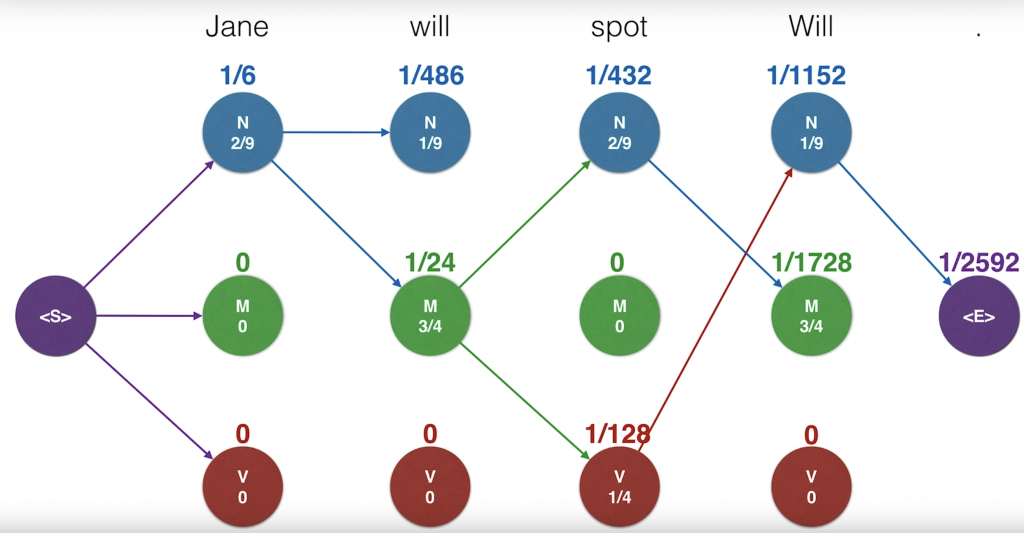
So how do we get our optimal path? Well, we’ll start from the end and trace backwards. Since each state only has one incoming edge, then this should give us a path that comes all the way from the beginning. And that path is the winning path.
and that’s it !!!!