LSTMs for Question Answering

LSTMs come in either or mode. In both modes, an LTSM processes a batch of stateless stateful
labeled training vectors. An LSTM works itself one step ( ) at a time through an input feature
vector, updating its cell state at each step. In stateless mode, after a sequence has been processed, the weights of the surrounding network layers are updated through back-propagation, and the cell state of the LSTM is reset. This means the LSTM will have to learn from a new sequence (vector) its gating weights (the various weights controlling which information is passed along, and which is forgotten) all over again; it’s notion of time is limited to one sequence.

Let’s quickly recap some issues pertaining to getting data into an LSTM layer. An LSTM
expects triples of data:

• (number of samples, time steps, features per timestep)

Simply put:

• number of samples: the number of samples in your data
• time steps: the length of the sequences fed to an LSTM. If we are feeding sentences to an LSTM, time steps addresses the words in every (length-padded) sentence.
• features: the dimensionality of the objects at every position of a sequence. For example: vectors of a certain dimension if we’re embedding words

Luckily, LSTMs can figure out these parameters themselves from a preceding input layer. Let’s go a little bit in details.Assume we have input data consisting of 10 features:

Suppose we apply a sliding window of two features over this sequence (treating it as a time sequence, with two features for each time tick), we obtain 10-2+1=9 subsequences:

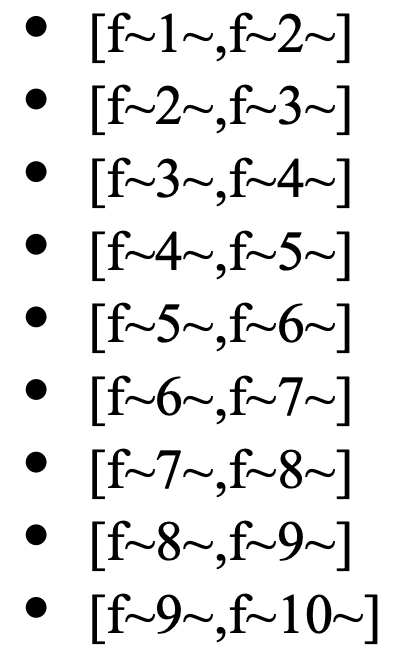
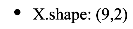
Assuming our data is initially represented as a nested array like:

with shape:

However, if we have another input layer preceding our LSTM layer, as in:

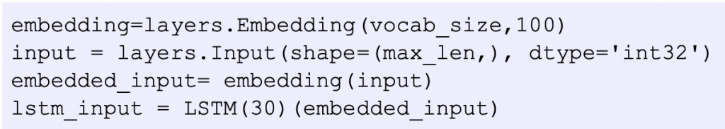
the LSTM layer, yielding an output vector of dimension 30, will deduce that it will receive batches of some unspecified size, consisting of a matrix of (max_len, 100) vectors: the embedding embeds a total of vocab_size vectors in a 100-dimensional vector space, and the input layer accepts input of size max_len. So, our LSTM layer cleverly assumes we have arranged our data in slices of max_len windows, with each cell of the windows containing a vector of dimension 100, and no further input shape specification is necessary at this point.

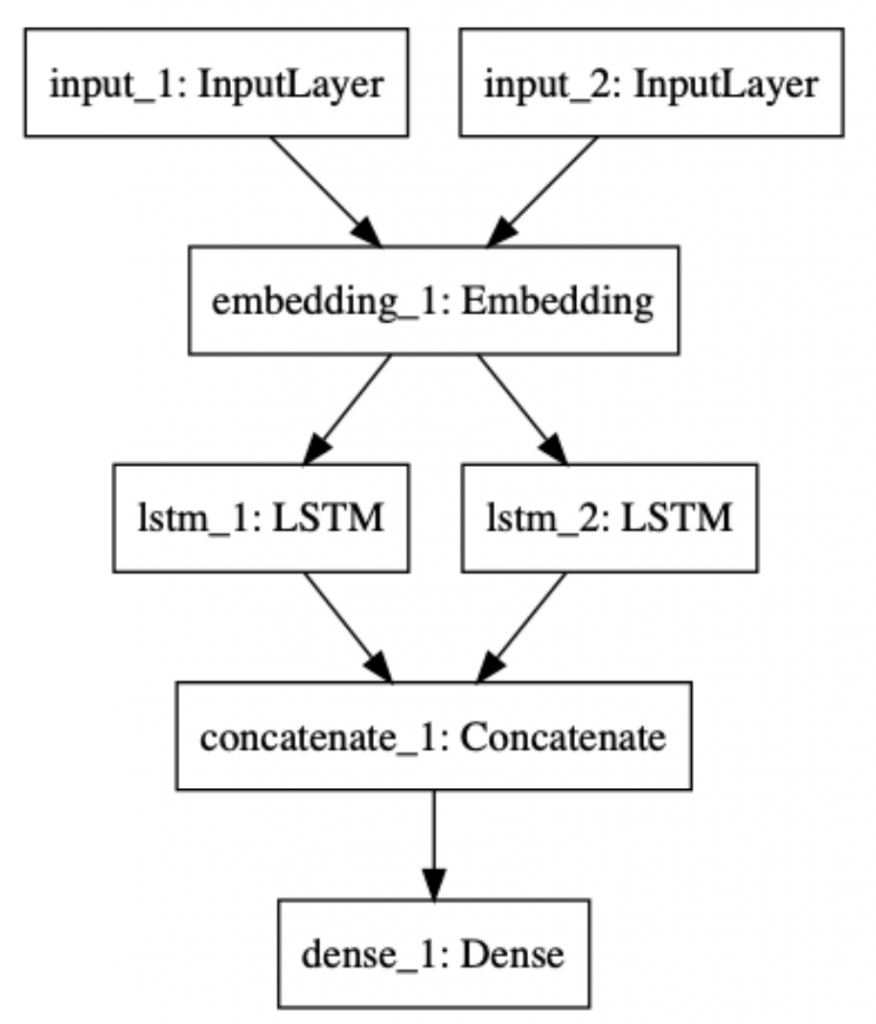
Our LSTM model is similar to the RNN model. It has two LSTM layers processing stories and questions, and the results (the output layers) are merged by concatenation. The following picture depicts its structure:

End-to-end memory networks for Question Answering

End-to-end memory networks embody responsive memory mechanisms. In the context of our Question-Answering task, rather than just teaching a network to predict an answer word index from a combined vector of facts and a question, these networks produce a memory response of a series of facts (a story) to the question posed, and use that response to weigh the facts vector. Only after this weighting has been carried out, the question is recombined with the weighted fact vector, and is used for predicting a word index, as before. So, we might say facts are weighted by the question prior to prediction. While looking like a modest step, this actually makes quite a difference. For one thing, explicit information about the match between question and facts is now being used for prediction. Recall that in our previous approaches, we merely lumped together facts and questions, without addressing the match between the two. How is this matching done, and why does it make a difference? Let’s take a look at the following picture

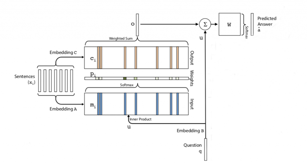
Facts (here called ‘sentences’) are embedded with an embedding A. The question q is embedded with an embedding B. Simultaneously, facts are embedded with a separate embedding C. The ‘response’ of the memory bank consisting of the embedded facts is computed by first deriving an inner product of the embedded facts with the embedded question, after which a softmax layer produces probalities based on the inner product. Notice that these are trainable probabilities that will be tuned during training through back-propagation. Finally, the probabilities are combined with the fact embedding produced by embedding with a weighted sum operation. This operation just adds the weights (probabilities) to the fact vector produced by C. At this point, the embedded question is combined through concatenation with the weighted sum. The result of this is sent to a final weights layer feeding into a dense output layer, encoding the word index of the answer.

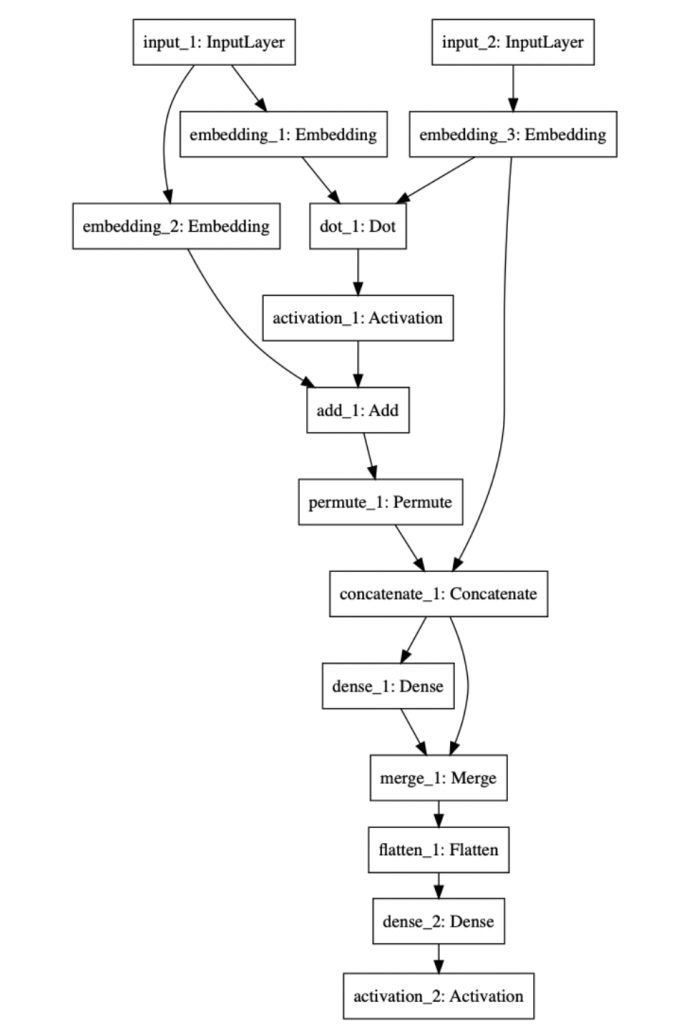
The following picture shows the model

The experimental code can be found at http://14.232.166.121:8880/lab andy > memory_QA , lstm_qa.ipynb and qa_mem.ipynb