Feature Extraction

Once we have our text ready in a clean and normalized form, we need to transform it into features that can be used for modeling. For instance, treating each document like a bag of words allows us to compute some simple statistics that characterize it. These statistics can be improved by assigning appropriate weights towards using a TF-IDF Scheme. This enables a more accurate comparison between documents. For certain applications, we may need to find numerical representations of individual words, and for that, we can use word embeddings, which are a very efficient and powerful method

Bag of Words

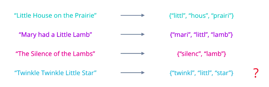
The first feature representation we’ll look at is called Bag of Words. The Bag of Words model treats each document as an un-ordered collection or bag of words. Here, a document is the unit of text that you want to analyze. For instance, if you want to compare essays submitted by students to check for plagiarism, each essay would be a document. If you want to analyze the sentiment conveyed by tweets, then each tweet would be a document. To obtain a bag of words from a piece of raw text

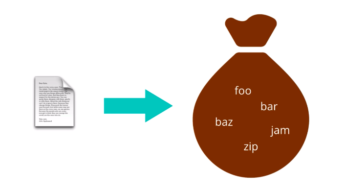
you need to simply apply appropriate text processing steps: cleaning, normalizing, splitting into words, stemming, lemmatization, etc…. And then treat the resulting tokens as an un-ordered collection or set. So, each document in your data set will produce a set of words. But keeping these as separate sets is very inefficient. They’re of different sizes, may contain different words, and are hard to compare. Also, whatever word occurs multiple times in a document?

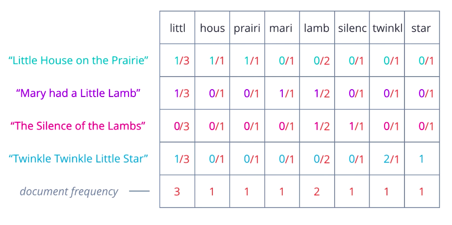
Is there a better representation you can think of? A more useful approach is to turn each document into a vector of numbers, representing how many times each word occurs in a document. A set of documents is known as a corpus, and this gives the context for the vectors to be calculated. First, collect all the unique words present in your corpus to form your vocabulary. Arrange these words in some order, and let them form the vector element positions or columns of a table, and assume each document is a row. Then count the number of occurrences of each word in each document and enter the value in the respective column. At this stage, it is easier to think of this as a Document-Term Matrix, illustrating the relationship between documents in rows, and words or terms in columns. Each element can be interpreted as a term frequency.

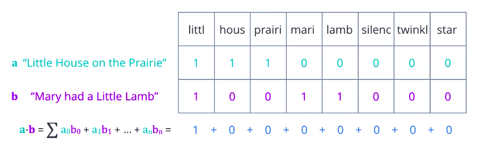
Now, consider what you can do with this representation. One possibility is to compare two documents based on how many words they have in common or how similar their term frequencies are. A more mathematical way of expressing that is to compute the dot product between the two row vectors, which is the sum of the products of corresponding elements. Greater the dot product, more similar the two vectors are. The dot product has one flaw, it only captures the portions of overlap. It is not affected by other values that are not uncommon. So, pairs that are very different can end up with the same product as ones that are identical. A better measure is cosine similarity, where we divide the dot product of two vectors by the product of their magnitudes or Euclidean norms. If you think of these vectors as arrows in some n-dimensional space, then this is equal to the cosine of the angle theta between them. Identical vectors have cosine equals one. Orthogonal vectors have cosine equal zero.

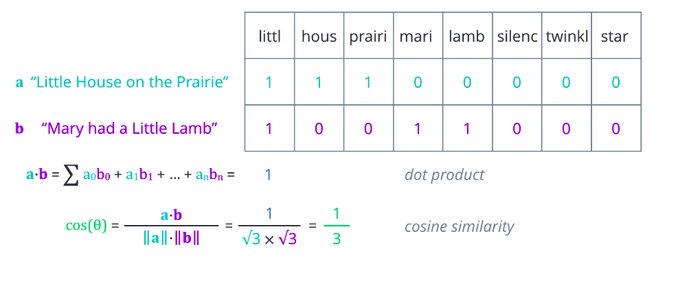
And for vectors that are exactly opposite, it is minus one. So, the values always range nicely between one for most similar, to minus one, most dissimilar.

TF-IDF

One limitation of the bag-of-words approach is that it treats every word as being equally important, whereas intuitively, we know that some words occur frequently within a corpus. For example, when looking at financial documents, cost or price may be a pretty common term.

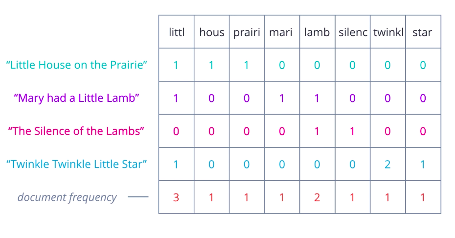
We can compensate for this by counting the number of documents in which each word occurs, this can be called document frequency, and then dividing the term frequencies by the document frequency of that term. This gives us a metric that is proportional to the frequency of occurrence of a term in a document, but inversely proportional to the number of documents it appears in. It highlights the words that are more unique to a document, and thus better for characterizing it.

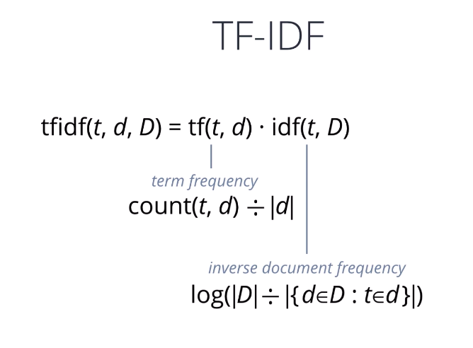
You may have heard of, or used, the TF-IDF transform before. It’s simply the product of two words, very similar to what we’ve seen so far, a term frequency and an inverse document frequency. The most commonly used form of TF-IDF defines term frequency as the raw count of a term, t, in a document, d, divided by the total number of terms in d, and inverse document frequency as the logarithm of the total number of documents in the collection, d, divided by the number of documents where t is present. Several variations exist that try to normalize, or smooth the resulting values, or prevent edge cases such as divide-by-zero errors. Overall, TF-IDF is an innovative approach to assigning weights to words that signify their relevance in documents.

One-Hot Encoding

So far, we’ve looked at representations that tried to characterize an entire document or collection of words as one unit. As a result, the kinds of inferences we can make are also typically at a document level, mixture of topics in the document, documents similarity, documents sentiment. For a deeper analysis of text, we need to come up with a numerical representation for each word. If you’ve dealt with categorical variables for data analysis or tried to perform multi-class classification, you may have come across this term, One-Hot Encoding.

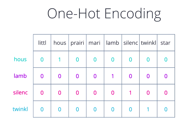
That is one way of representing words, treat each word like a class, assign it a vector that has one in a single pre-determined position for that word and zero everywhere else. Looks familiar? Yeah, it’s just like the bag of words idea, only that we keep a single word in each bag and build a vector for it.

Word Embeddings

One-hot encoding usually works in some situations but breaks down when we have a large vocabulary to deal with, because the size of our ward representation grows with the number of words. What we need as a way to control the size of our word representation by limiting it to a fixed-size vector. In other words, we want to find an embedding for each word in some vector space and we wanted to exhibit some desired properties.

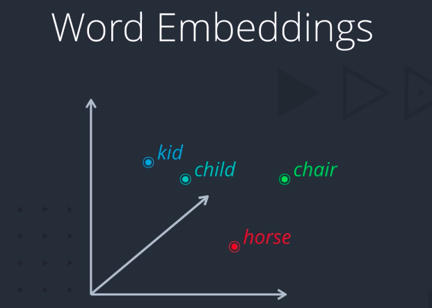
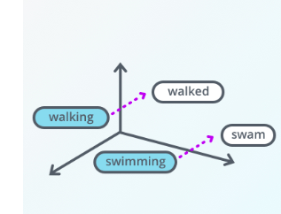
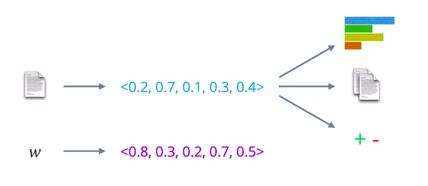
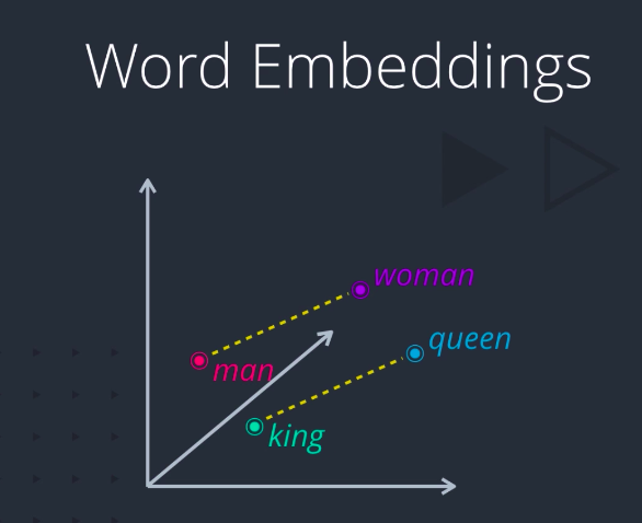
For example, if two words are similar in meaning, they should be closer to each other compared to words that are not. And if two pairs of words have a similar difference in their meanings, they should be approximately equally separated in the embedded space. We could use such a representation for a variety of purposes like finding synonyms and analogies, identifying concepts around which words are clustered, classifying words as positive, negative, neutral, etc. By combining word vectors, we can come up with another way of representing documents as well.

Word2Vec

Word2Vec is perhaps one of the most popular examples of word embeddings used in practice. As the name Word2Vec indicates, it transforms words to vectors. But what the name doesn’t give away is how that transformation is performed. The core idea behind Word2Vec is this, a model that is able to predict a given word, given neighboring words, or vice versa, predict neighboring words for a given word is likely to capture the contextual meanings of words very well.

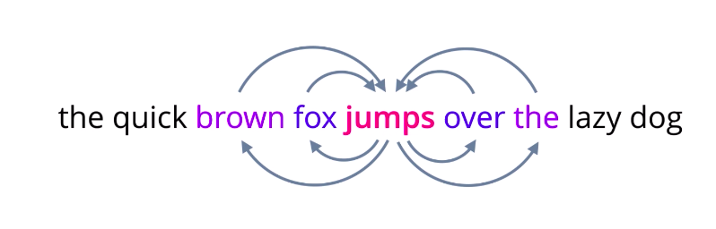
And these are, in fact, two flavors of Word2Vec models, one where you are given neighboring words called continuous bag of words, and the other where you are given the middle word called Skip-gram. In the Skip-gram model, you pick any word from a sentence, convert it into a one-hot encoded vector and feed it into a neural network or some other probabilistic model that is designed to predict a few surrounding words, its context. Using a suitable loss function, optimize the weights or parameters of the model and repeat this till it learns to predict context words as best as it can.

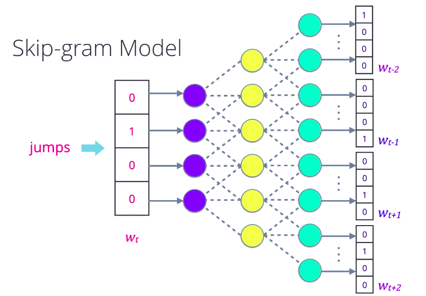
Now, take an intermediate representation like a hidden layer in a neural network. The outputs of that layer for a given word become the corresponding word vector. The Continuous Bag of Words variation also uses a similar strategy. This yields a very robust representation of words because the meaning of each word is distributed throughout the vector. The size of the word vector is up to you, how you want to tune performance versus complexity. It remains constant no matter how many words you train on, unlike Bag of Words, for instance, where the size grows with the number of unique words. And once you pre-train a large set of word vectors, you can use them efficiently without having to transform again and again, just store them in a lookup table. Finally, it is ready to be used in deep learning architectures. For example, it can be used as the input vector for recurrent neural nets. It is also possible to use RNNs to learn even better word embeddings. Some other optimizations are possible that further reduce the model and training complexity such as representing the output words using Hierarchical Softmax, computing loss using Sparse Cross Entropy.

GloVe

Word2vec is just one type of forward embedding. Recently, several other related approaches have been proposed that are really promising. GloVe or global vectors for word representation is one such approach that tries to directly optimize the vector representation of each word just using co- occurrence statistics, unlike word2vec which sets up an ancillary prediction task. First, the probably that word j appears in the context of word i is computed, pj given i for all word pairs ij in a given corpus. What do we mean by j appears in context of i? Simply that word j is present in the vicinity of word i, either right next to it, or a few words away. We count all such occurrences of i and j in our text collection, and then normalize account to get a probability. Then, a random vector is initialized for each word, actually two vectors. One for the word when it is acting as a context, and one when it is acting as the target. So far, so good. Now, for any pair of words, ij, we want the dot product of their word vectors, w_i times w_j, to be equal to their co-occurrence probability. Using this as our goal and a suitable last function, we can iteratively optimize these word vectors.

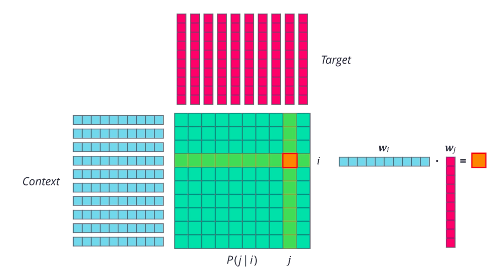
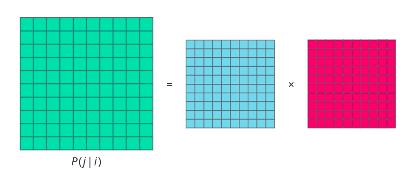
The result should be a set of vectors that capture the similarities and differences between individual words. If you look at it from another point of view, we are essentially factorizing the co-occurrence probability matrix into two smaller matrices. This is the basic idea behind GloVe.

All that sounds good, but why co-occurrence probabilities? Consider two context words, say ice and steam, and two target words, solid and water. You would come across solid more often in the context of ice than steam, right? But water could occur in either context with roughly equal probability. At least, that’s what we would expect. Surprise. That’s exactly what co-occurrence probabilities reflect.

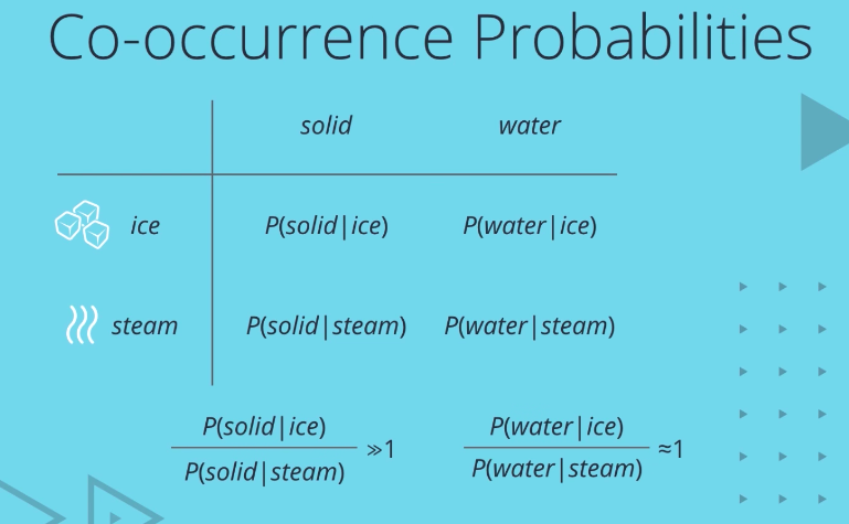
Given a large corpus, you’ll find that the ratio of P solid given ice to P solid given steam is much greater than one, while the ratio of P water given ice and P water given steam is close to one. Thus, we see that co-occurrence probabilities already exhibit some of the properties we want to capture. In fact, one refinement over using raw probability values is to optimize for the ratio of probabilities. Now, there are a lot of subtleties here, not the least of which is the fact that the co-occurence probability matrix is huge. At the same time, co-occurrence probability values are typically very low, so it makes sense to work with the log of these values

Embeddings for Deep Learning

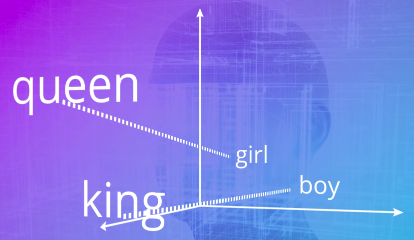
The embeddings are fast becoming the de facto choice for representing words, especially for use and deep neural networks. But why do these techniques work so well? Doesn’t it seem almost magical that you can actually do arithmetic with words, like woman minus man plus king equals queen?

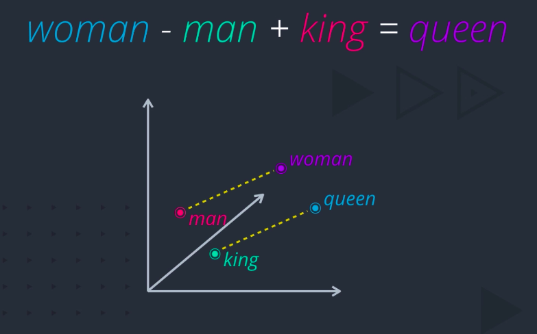
The answer might lie in the distributional hypothesis, which states that words that occur in the same contexts tend to have similar meanings. For example, consider this sentence

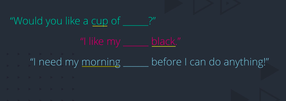
What are you thinking? Tea? Coffee? What give you the hint? Cup? Black? Morning? But it could be either of the two, right? And that’s the point. In these contexts, tea and coffee are actually similar. Therefore, when a large collection of sentences is used to learn in embedding, words with common context words tend to get pulled closer and closer together. Of course, there could also be contexts in which tea and coffee are dissimilar

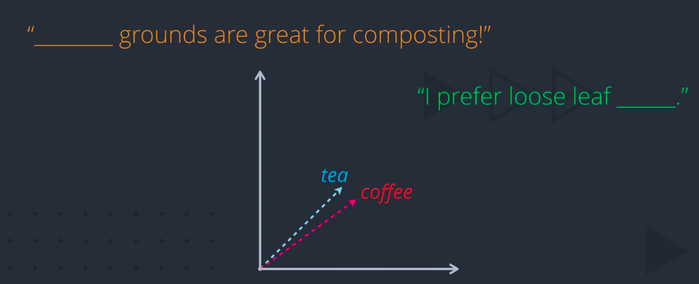
How do we capture these similarities and differences in the same embedding? By adding another dimension. Let’s see how. Words can be close along one dimension. Here, tea and coffee are both beverages, but separated along some other dimension. Maybe this dimension captures all the variability among beverages. In a human language, there are many more dimensions along which word meanings can vary. And the more dimensions you can capture in your word vector, the more expressive that representation will be.