Topic Modeling
Intro
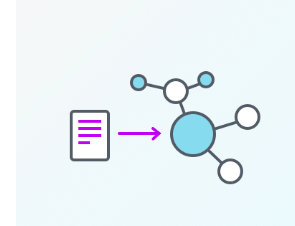
The bag-of-words approach tries to represent documents in a dataset directly using the words that appear in them. But often, these words are predicated on some underlying parameters are very among documents such as a topic being discussed. In this blog, we’ll begin with discussing this hidden or latent variables. Then, we’ll look at a specific technique used to estimate them called Latent Dirichlet Allocation. Finally, you’ll get to apply the knowledge you’ve learned to perform topic modeling on a collection of documents.
Bag of Words
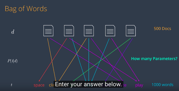
Let’s start with a regular bag of words model. If you think about the Bag of Words model graphically, it represents the relationship between a set of document objects and a set of word objects. It’s very simple. Let’s say we’ve got an article like this one and we look at what words are in that article. We’ll assume that we do the correct stemming and text processing so that we only look at the important words. So this article has three words namely space, vote and explore. The word space appears twice, the word vote appears once and the word explore or it’s related words like exploration appears three times. To find the probabilities of each word appearing in the article, we divide by the total number of words and we get some probabilities. This gives us three parameters. Now to add some notation, we call documents d, our words or terms t and the parameters are precisely the probability of a word appearing in the documents, so that is P of t given d. Specifically this parameter say, p(t|d) for any given document d and observed term t. How likely is it that the document d generated the term t? So now we do this for a bunch of documents and a bunch of words. We draw all these probabilities. And let’s have a quiz Let’s say we have 500 documents and 1000 unique words How many parameters are in this model?
Latent Variables
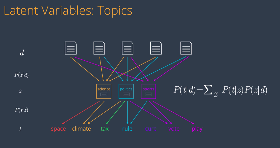
Well, the answer is, we need one arrow for each pair document word. Since we have 500 documents and 1,000 words, the number of parameters is the number of documents times the number of words. This is 500 times 1,000, which is 500,000. This is too many parameters to figure out. Is there any way we can reduce this number and still keep most of the information? The answer is yes. We can reduce the number of parameters and still catch most of the information. We’ll do this by adding to the model the notion of a small set of topics or latent variables that actually drive the generation of words in each document. So, in this model, any document is considered to have an underlying mixture of topics associated with it. Similarly, a topic is considered to be a mixture of terms that is likely to generate. In here, we have say three topics: Science, politics, and sports. So now, there are two sets of parameters of probability distributions that we need to compute. The probability of a topic given a document d or P(z/d) and the probability of a term P given a topic z, or P(t/z). Our new probability of a document given a term can be expressed as a sum over the two previous probabilities.
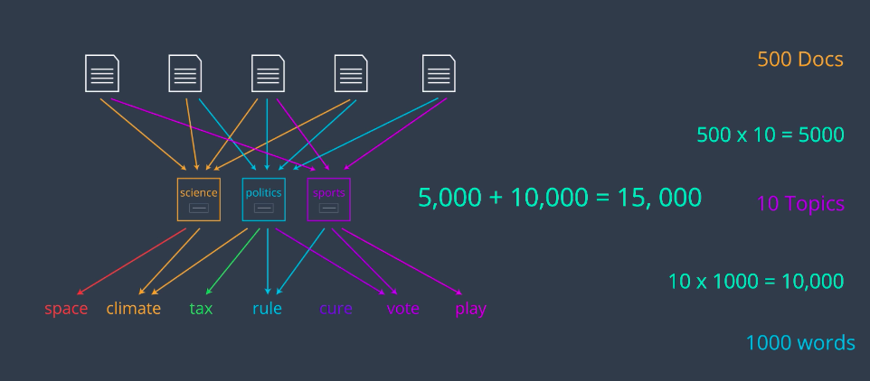
So, it’s time for another quiz. If we have 500 documents, 10 topics and 1,000 words, how many parameters does this new model have?
Matrix Multiplication
well, let’s see. The first part has 500 times 10 parameters, which is 5,000. The second part has 10 times 1,000, which is 10,000. So, together, they have 15,000 parameters. This is much better than 500,000. This is called Latent Dirichlet Allocation or LDA for short.
An LDA is an example of matrix factorization. We’ll see how. The idea is the following: we go from this Bag of Words model in the left to the LDA model in the right.
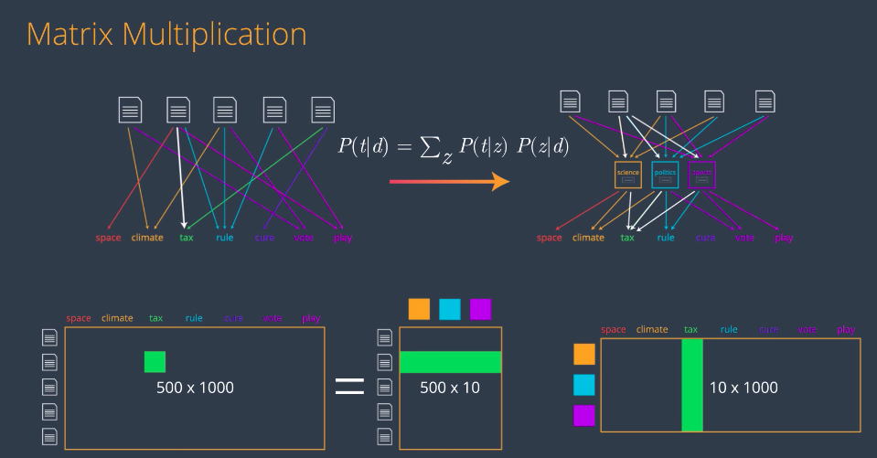
The Bag of Words model in the left basically says our probability of, say, the word tax being generated by the second document is the label of this arrow. On the LDA model in the right, that probability is calculated by these arrows by multiplying the P of t given z on the top by the corresponding P of z given d on the bottom and adding them. This formula reminds us a bit of matrix multiplication in the following way. We can put all the probabilities in the left model on a big matrix, then the idea is to write this big bag of words matrix as a product of a tall skinny matrix indexed by documents and topics with a wide flat matrix indexed by topics and terms. In this case, the entry corresponding to say the second document and the term “tax” in the Bag of Words matrix will be equal to the inner product of the corresponding row and column in the matrices on the right. And as before, if the matrices are big, say if we have 500 documents, 10 topics and 1,000 terms, the Bag of Words matrix has 500,000 entries, whereas the two matrices in the topic model combined have 15,000 entries. But aside from being much simpler, the LDA model has a huge advantage that it gives us a bunch of topics that we can divide the documents on. In here we’re calling them science, politics, and sports, but in real life, the algorithm will just throw some topics and it’ll be up to us to look at the associated words and decide what is the common topic of all these words. We’ll keep them as science, politics, and sports for clarity, but think of them as topic 1, topic 2, and topic 3.
Matrices
So, the idea for building our LDA model will be to factor are Bag of Words matrix on the left into two matrices
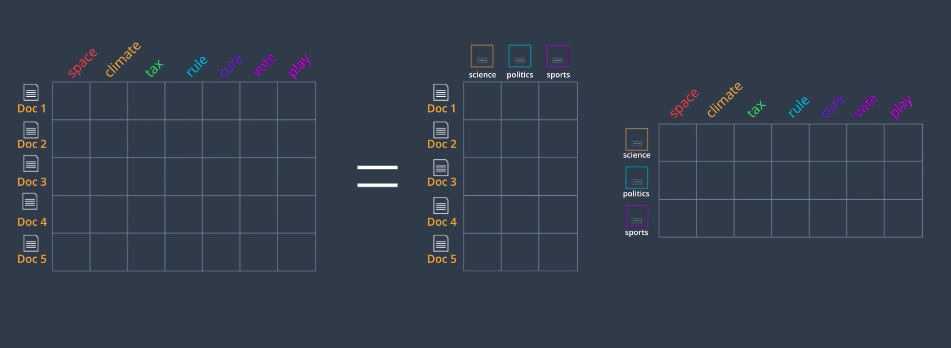
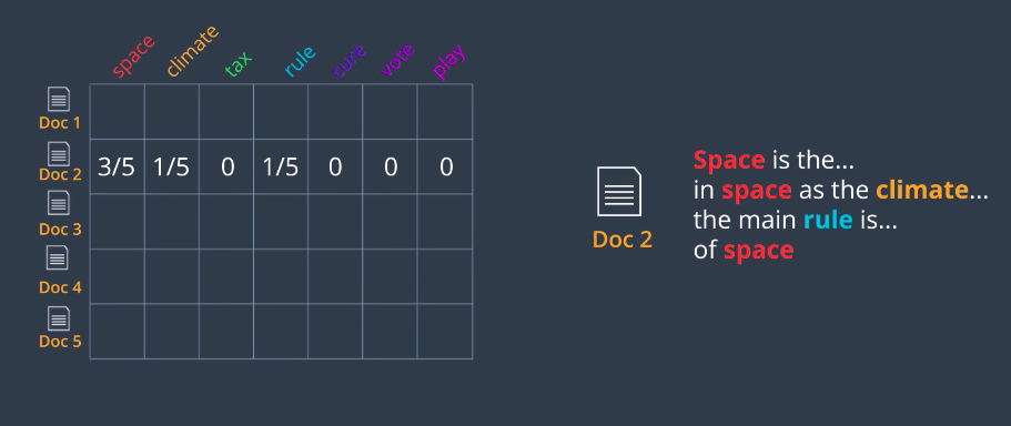
one indexing documents by topic and the other indexing topics by word. Here’s how we calculate our Bag of Words matrix. Let’s say we have a document, Document two which has the words space three times, climate and rule once each and no other words. Remember that we process this document and extracted the important words so things like is, the, and are not counted. We write these numbers in the corresponding row. Now to find the probabilities, we just divide by the row sum and we get three-fifths, one-fifth, one-fifth, and zeros for the rest. That’s our Bag of Words matrix.
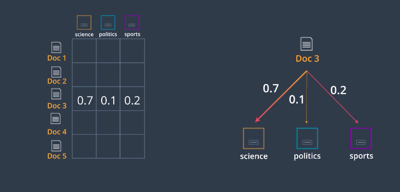
Our document topic matrix is as follows; Let’s say we have a document say Document three, and let’s say we have a way to figure out that Document three is mostly about science and a bit about sports and politics. Let’s say it’s 70 percent about science, 10 percent about politics, and 20 percent about sports. So, we just record these numbers in the corresponding row and that’s how we obtain this matrix.
The topic term matrix is similar. Here we have a topic, say politics, and let’s say we can figure out the probabilities that words are generated by this topic. We take all this probabilities we should add to one and put them in the corresponding row. As we saw, the product of these two matrices is the Bag of Word matrix. Well, this is not exact but the idea is to get really close. If we can find two matrices whose product is very close to the Bag of Word matrix, then we’ve created a topic model. But I still haven’t told you how to calculate the entries in these two matrices. Well, one way is using the traditional matrix factorization algorithm. However, these matrices are very special. For ones, the rows add up to one. Also if you think about it, there’s a lot of structure coming from a set of documents, topics and words. So, what we’ll do is something a bit more elaborate than matrix multiplication. The basic idea is the following: the entries in the two topic modeling matrices come from some special distributions. So, we’ll embrace this fact and work with these distributions to find these two matrices.
Beta Distribution
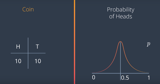
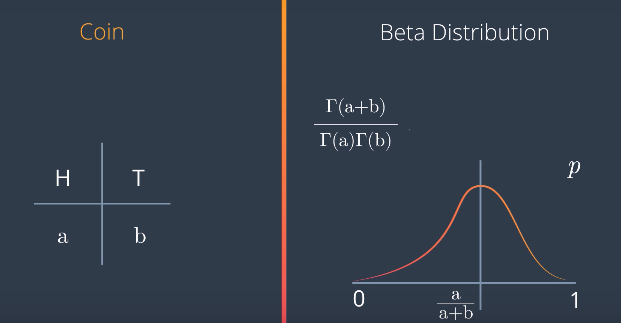
So, let’s go to probability distributions. Let’s say we have a coin, and we toss it twice. Let’s say we get one heads and one tails. What would we think about this coin? Well, it could be a fair coin, right? It could also be slightly biased towards either heads or tails. We don’t have enough data to be sure. So, let’s say that our verdict is that we think it’s fair, but with not much confidence. So, let’s think of the probability p that this coin lands on heads. With a little bit of confidence, p is one half but it could be a lot of other values.
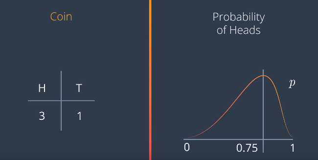
Now, let’s say we toss a coin four times, and we get heads three times, and tails one. The probability distribution for p is now centered at 0.75 since we get three heads out of four tries. But also with not much confidence. So, it’s a graph like this.
But if we toss it 400 times, and it lands on heads 300, then we’re much more confident that the value of p is close to 0.5. Therefore, the probability distribution for p is something like this with a huge peak at at 0.75, and almost flat everywhere else. This is called a Beta distribution, and it works for any values of A and B. If we get heads A times and tails B times, the graph looks like this with a peak at A over A+B The formula is this
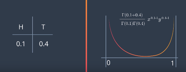
the Gamma function is that it also takes values in between. So, we can define things like Gamma of 5.5, and it will be something between 24 and 120. So, what happens if we have values that are not integers like say, 0.1 for heads, and 0.4 for tails. This makes no sense since we can get 0.1 heads and 0.4 tails. But that’s okay for the Beta distribution. We just need to grab the right formula using the Gamma function. For values smaller than one, like 0.1 and 0.4, we get this graph. That means p is much more likely to be either close to zero or close to one than to be in the middle.
Latent Dirichlet Allocation
Now, a Multinomial Distribution is simply a generalization of the binomial distribution to more than two values. For example, let’s say we have newspaper articles and three topics: science, politics, and sports. Let’s say each topic is assigned randomly to the articles, and when we look, we have three science articles, six politics articles, and two sports articles. So, for a new article, what would the probability be that it’s science, politics, or sports? We would imagine it’s a bit higher for politics and science, and higher for science and sports. This is not for sure, but it’s likely to happen.
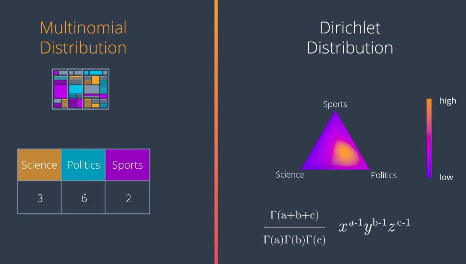
So now, these three probabilities live in a triangle where if we pick a point than any of the corners, it means the probability for that topic is one, and the others are zero, and if we pick it in the middle, then the probabilities are similar for the three topics. So, maybe the probability density distribution for these three probabilities will be like this one here, since articles are more likely to be politics than anything else, and less likely to be sports than anything else. This probability density distribution is calculated with a generalization of the formula for the Beta distribution given here. It’s called a Dirichlet distribution.
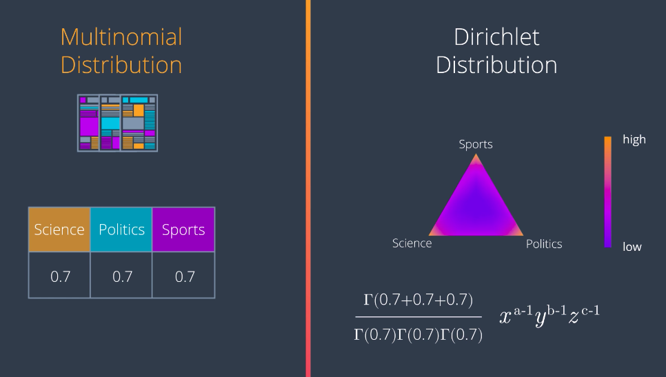
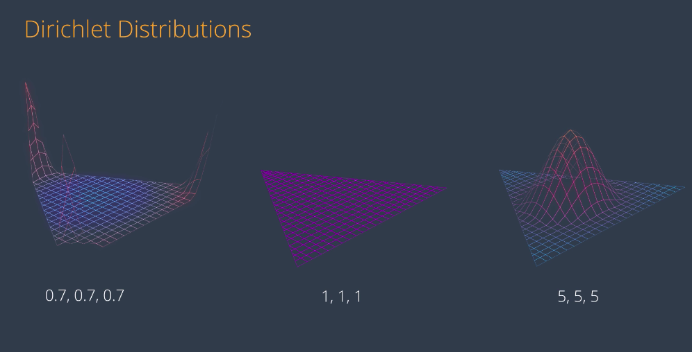
Again, there is no reason for these numbers to have to be integers. For example, if we have 0.7, 0.7, and 0.7, this is the Dirichlet distribution. It’s hard to see, but the density function is very high when we get really close to the corners of the triangle. Meaning that any point picked randomly from this distribution is very likely to fall either at the science, politics, or sports corners, or at least close to any of the edges, and very unlikely to be somewhere in the middle.
Here are some samples of Dirichlet distributions with different values. Notice that if the values are large, the density function is high in the middle, and if they’re small, it’s higher in the corners. If the values are different from each other, then the high part moves towards the smaller values, and away from the larger values. This is how they look in 3D. So, notice that if we want a good topic model, we need to pick small parameters like the one on the left. This is how we’ll pick our topics from now on.
Latent Dirichlet Allocation
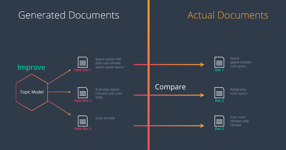
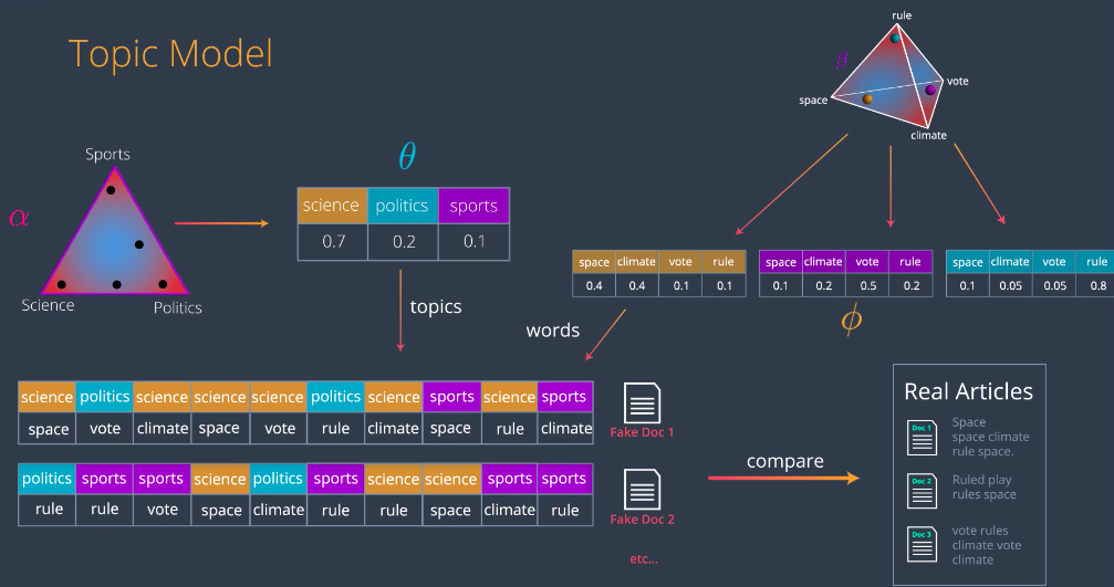
So, now let’s build our LDA model. The idea is the following; We’ll have our documents here, let’s say these three documents, and then we’ll generate some fake documents, like this three over here. The way we generate them is with the topic model, and then what we do is we compare the generated documents with the real ones. This will tell us how far we are from creating the real documents with our model. Like in most Machine Learning algorithms, we learned from these error and we’ll be able to improve her topic model. This is what we’ll do, in the paper the topic model is drawn like this, this looks complicated but we’ll analyze this in the next few videos
Sample a Topic
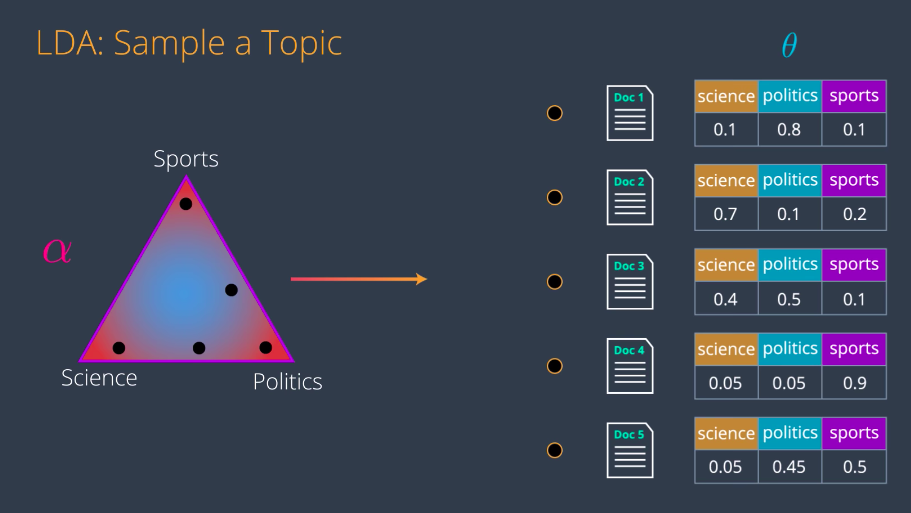
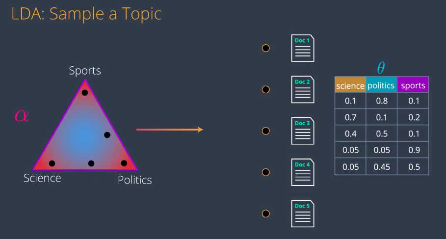
Let’s start by picking some topics for our documents. We start with some declared distribution with parameters Alpha. And the parameters should be small for the distribution to be spiky towards the sites. Which means, if we pick a point somewhere in the distribution, it will most likely be close to a corner or at least to an edge. Let’s say we pick this point close to the politics corner which generates the following values 0.1 for Science, 0.8 for politics and 0.1 for sports.
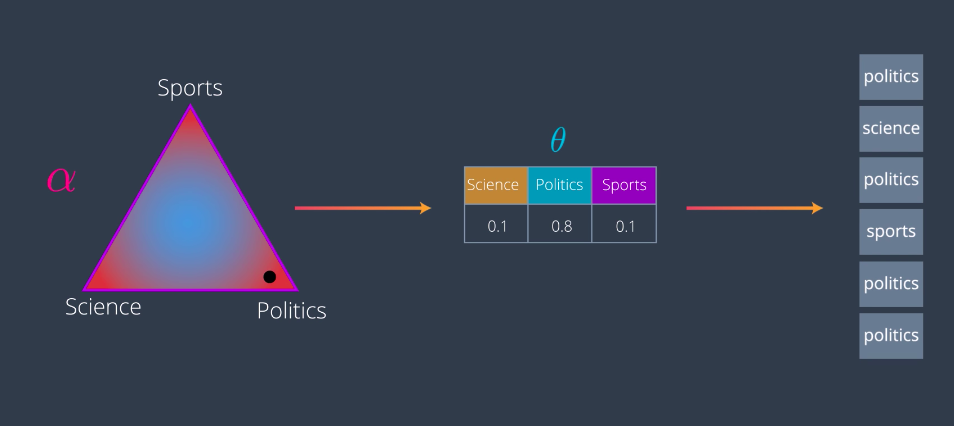
These values represent a mixture of topics for this particular document. They also give us a multinomial distribution theta. Now from this distribution, we’ll start picking topics. That means the topics we’ll pick are Science with a 10 percent probability, politics with an 80 percent probability and sports with a 10 percent probability. So, we’ll pick some topics say politics, science, politics, sports etc. And we do this for several documents. So, each document is a point in this declared distribution. Let’s say document one is here which gives us this multinomial distribution. Then, document two is here which gives us this other one, and we’ll do this for all the documents.
And now, we merge all these vectors to get the first matrix. The matrix that indexes documents with their corresponding topics.
Sample a Word
Now, we’ll do the same thing for topics and words. Let’s say for the sake of visualization that we only have four words: space, climate, vote, and rule. Now we have a different distribution, beta. This one is similar to the previous one but it is three-dimensional, is not around a triangle but it’s around a simplex. Again, the red parts are high probability and the blue parts are low probability.
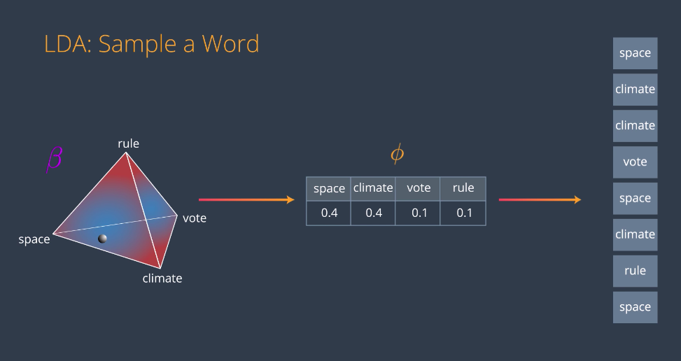
If we had more words, we would still have a very clear distribution except it would be in a much higher dimensional simplex. This is why we picked four words because we can visualize that simplex in 3D. So, in this distribution beta, we pick a random point and it will very likely be close to a corner or an edge. Let’s say it’s here. This point generates the following multinomial distribution, 0.4 for space, 0.4 for climate, and 0.1 for vote and rule. This multinomial distribution we’ll be called phi and it represents the connections between the words and the topic. Now from this distribution, we will sample random words which are 40 percent likely to be space, 40 for climate, 10 for vote and 10 for rule. The words could look like this. Now we do this for every topic. So, Topic 1 is say around here close to Space and Climate, topic 2 is here close to vote, and on topic 3 is here close to rule. Notice that we don’t know what topics they are, we just know them as topic 1, 2, and 3.
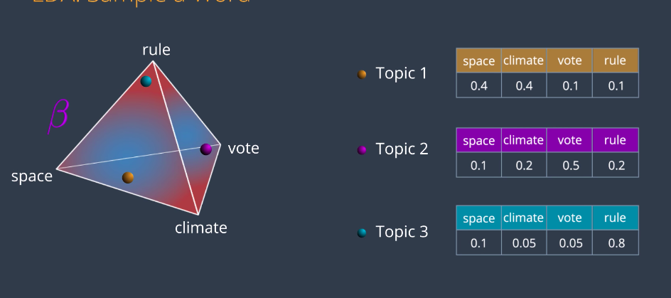
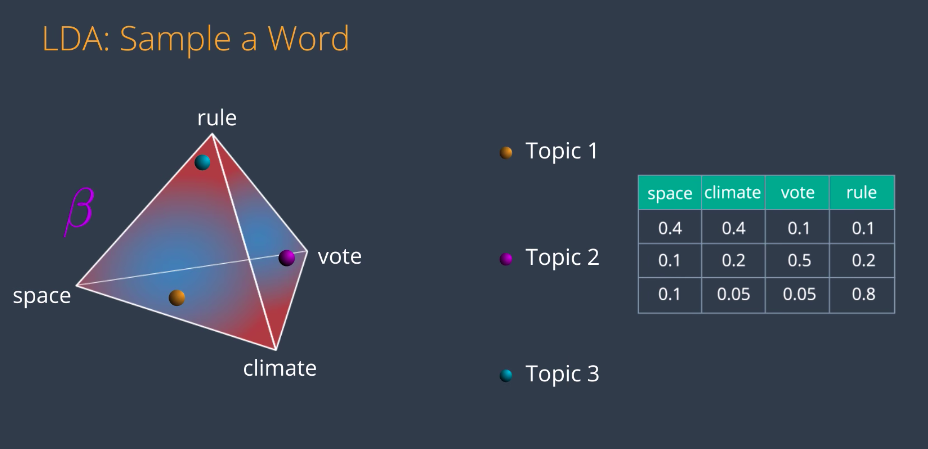
After some inspection, we can infer that topic 1 being close to Space and Climate must be science. Similarly, topic 2 being close to vote could be Politics and topic 3 being close to rule could be sports. But this is something that we’d be doing at the end of the model. And as a final step, we join these three together to obtain our other matrix in the LDA model.
Combining the Models
So, now let’s put this all together and study how to get these two matrices in the LDA model based on their respective dirichlet distributions. The rough idea is as we just saw, the entries from the first matrix come from picking points in the distribution alpha. The interest from the second matrix come from from picking points in distribution beta. The idea is to find the best locations of these points to get the best factorization of the matrix. The best locations of these points will give us precisely the topics we want. Let’s generate some documents, in order to compare them with the originals. We started with dirichlet distribution for topics alpha. From here, we draw some points corresponding to all the documents. Let’s start by drawing one of them. This point will give some values for each of the three topics, which will generate a multivariate distribution theta. This is the mixture of topics, corresponding to document one. Now, let’s generate some words for document one as follows. From theta, we draw some topics. How many topics? This is a bit out of the scope, but the idea is that we’ll have a Poisson variable to tell us how many. Just think of yet another parameter in this model. So, we draw some topics based on the probability is given by this distribution, which means, we’ll draw science with a 0.7 probability, politics with 0.2, and sports with 0.1. Now, we’ll associate words to these topics. How? Using the words dirichlet distribution beta. In this distribution, we locate the topic somewhere, and from each of these dots, we obtain a distribution of the words, are generated by each of the topics. For example, topic one science, generates the word space with 0.4 Climate with 0.4, vote with 0.1, probability. and rule with 0.1 probability These distributions are called phi.
Now, for each of the topics we’ve chosen, we’ll pick a word associated to it using the multivariate distribution phi. For example, for the first topic we have science. We look at the science row in the phi distribution and pick a word out there. For example, space. So, space is the first word in document one. We do this for every one of these topics and then generate words from our first generated document. Let’s call it “fake document one”. We do this process again, drawing another point from the alpha distribution, getting another multivariable distribution theta, which generates new topics which from beta generate new words and that’s “fake document two”. We go on and on, generating many documents. Now, it’s time to compare them with originals. What we’ll do is we want to use maximum likelihood to figure out the arrangements of points which will give us the real articles with the highest probability. In summary, here’s what we’re doing. We have the two dirichlet distributions, alpha and beta. From the distribution alpha, we pick some documents and from distribution beta, we pick some topics. We use these two combined to create some fake articles. Then we compare them to the real articles. The probability of obtaining the real articles, of course is really small, but there must be some arrangement of points in the above distributions that maximizes this probability. Our goal is to find this arrangement of points and that will give us the topics. In the same way that we train many algorithms in machine learning, there will be an error that will tell us how far we are from generating the real articles. The error will back propagate all the way to the distributions, giving us a gradient that will tell us where to move the points in order to reduce this error. So, we move the points as indicated and now we’ve obtained a slightly better model. Doing this repeatedly, will give us a good enough arrangement on the points. Naturally, a good arrangement of the points will give us some topics. The dirichlet distribution alpha, will tell us what articles are associated to these topics and the dirichlet distribution beta, will tell us what words are associated to these topics. We can go a bit further and actually backpropagate the error
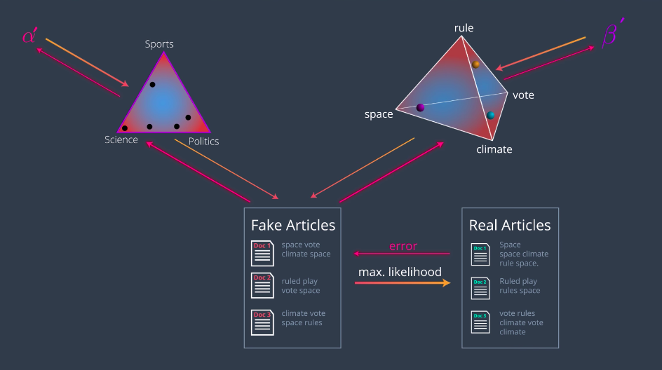
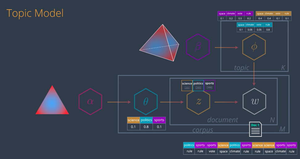
all the way to alpha and beta, obtaining not only better point arrangements but actually better distributions, alpha and beta prime. That’s it. That’s how latent dirichlet analysis works. If you want to understand the diagram and the paper, here it is. All we need to know, what the alpha is the topics distribution. Beta is the words distribution, theta and phi, are the multivariate distributions drawn from them, Z are our topics and W, are the documents obtained by combining these two.
The practice notebook for the topic modeling can be found at http://14.232.166.121:8880/lab andy > topic-modeling > latent_dirichlet_allocation.ipynb