Language Models
“Being able to predict the future is not always a good thing. Cassandra of Troy had the gift of foreseeing but was cursed by Apollo that no one would believe her predictions. Her warnings of the destruction of Troy were ignored and — well, let’s just say that things didn’t turn out great for her.”
Models that assign probabilities to sequences of words are called language models or LMs
LMs could predict that the following sequence has a much higher probability of appearing in a text:
“all of a sudden I notice three guys standing on the sidewalk”
than does this same set of words in a different order:
“on guys all I of notice sidewalk three a sudden standing the”
N-Grams
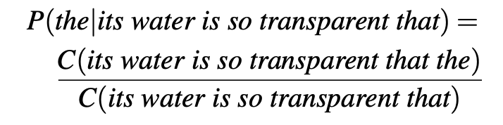
Let’s begin with the task of computing P(w|h), the probability of a word w given some history h. Suppose the history h is “its water is so transparent that” and we want to know the probability that the next word is the:

One way to estimate this probability is from relative frequency counts: take a very large corpus, count the number of times we see its water is so transparent that, and count the number of times this is followed by the. This would be answering the question “Out of the times we saw the history h, how many times was it followed by the word w”, as follows:
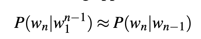
The bigram model, for example, approximates the probability of a word given all the previous words by using only the conditional probability of the preceding word . In other words, instead of computing the probability:
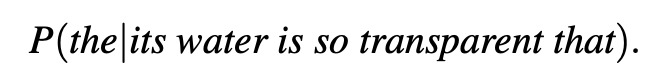
we approximate it with the probability:
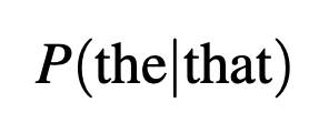
When we use a bigram model to predict the conditional probability of the next word, we are thus making the following approximation:
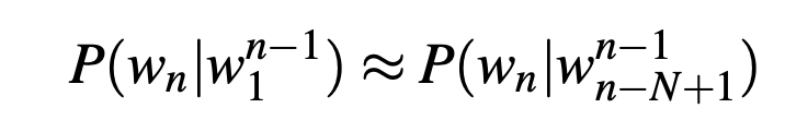
The assumption that the probability of a word depends only on the previous word Markov is called a Markov assumption. Markov models are the class of probabilistic models that assume we can predict the probability of some future unit without looking too far into the past. We can generalize the bigram (which looks one word into the past) n-gram to the trigram (which looks two words into the past) and thus to the n-gram (which looks n−1 words into the past). Thus, the general equation for this n-gram approximation to the conditional probability of the next word in a sequence is:
Let’s work through an example using a mini-corpus of three sentences. We’ll first need to augment each sentence with a special symbol at the beginning of the sentence, to give us the bigram context of the first word. We’ll also need a special end-symbol
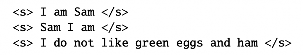
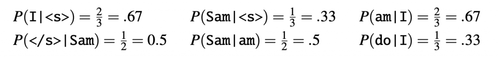
Here are the calculations for some of the bigram probabilities from this corpus:
Evaluating Language Models:
The best way to evaluate the performance of a language model is to embed it in an application and measure how much the application improves. Such end-to-end evaluation is called extrinsic evaluation.
Unfortunately, running big NLP systems end-to-end is often very expensive. Instead, it would be nice to have a metric that can be used to quickly evaluate potential improvements in a language model. An intrinsic evaluation metric is one that measures the quality of a model independent of any application
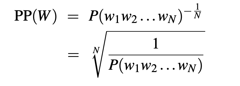
Perplexity
In practice we don’t use raw probability as our metric for evaluating language models, but a variant called perplexity
Neural Language Models
Neural net-based language models turn out to have many advantages over the ngram language models.
Among these are that neural language models don’t need smoothing, they can handle much longer histories, and they can generalize over contexts of similar words. For a training set of a given size, a neural language model has much higher predictive accuracy than an n-gram language model Furthermore, neural language models underlie many of the models we’ll introduce for tasks like machine translation, dialog, and language generation.
Window-Based Language Models
In neural language models, the prior context is represented by embeddings of the previous words. Representing the prior context as embeddings, rather than by exact words as used in n-gram language models, allows neural language models to generalize to unseen data much better than n-gram language models
The first neural language model was proposed by Bengio et al. (2003)
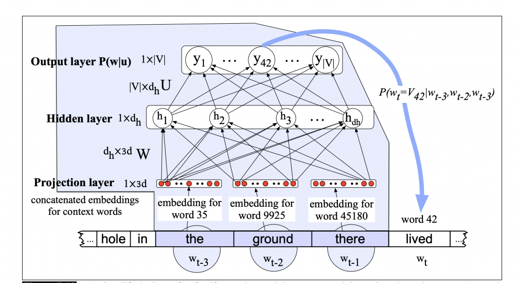
This figure shows a sketch of this simplified FFNNLM with N=3; we have a moving window at time t with an embedding vector representing each of the 3 previous words (words wt−1, wt−2, and wt−3). These 3 vectors are concatenated together to produce x, the input layer of a neural network whose output is a soft-max with a probability distribution over words. Thus y42, the value of output node 42 is the probability of the next word wt being V42, the vocabulary word with index 42.
RNN-Based Language Models
Unlike the conventional translation models, where only a finite window of previous words would be considered for conditioning the language model, Recurrent Neural Networks (RNN) are capable of conditioning the model on all previous words in the corpus.
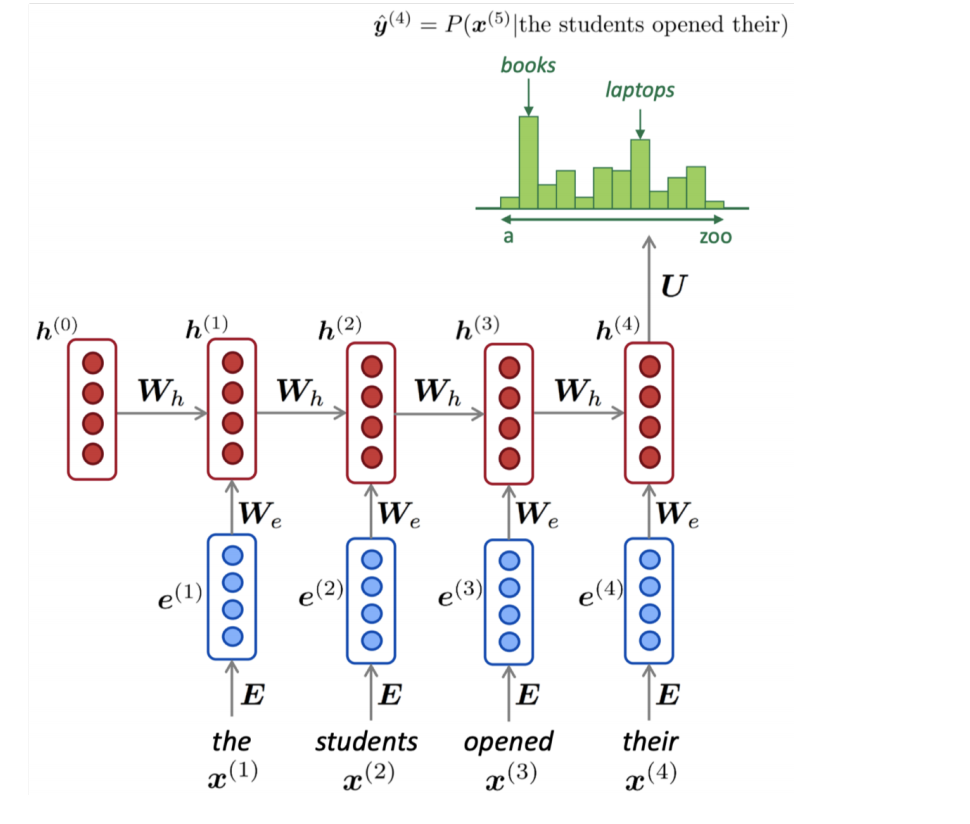
An example of an RNN language model is shown in this figure. The final softmax over the vocabulary shows us the probability of various options for token x (5) , conditioned on all previous tokens. The input could be much longer than 4–5 tokens.
You can take a look at a more detail explanations for RNN, LSTM in the following posts: